4.4. Change in the extent of water-related ecosystems over time [6.6.1]
This exercise introduces a possible workflow to calculate the SDG indicator 6.6.1, which tracks how different types of water-related ecosystems change in extent over time. The indicator captures data on different types of freshwater ecosystems and measures their extent change. The indicator 6.6.1 is complex and it focuses on more aspects than just the change in the spatial extent of permanent freshwater, but for the exercise’s simplicity sake just this unit of measure will be presented in this section. This index will be presented by the percentage change (∆) in the area of permanent waters. We will calculate ∆ as:
\(∆ = \frac{(α - β) + (ρ - σ)}{ε + β + σ}\), where:
α - new permanent water (conversion of a no water place into a permanent water place)
β - lost permanent water (conversion of a permanent water place into a no water place)
ρ - seasonal to permanent (conversion of seasonal water into permanent water)
σ - permanent to seasonal (conversion of permanent water into seasonal water)
ε - permanent water surfaces (where permanent water is always observed)
The numerator represents the change trends of the permanent water (if the numerator is positive it means that the area of permanent water places increased with respect to the beginning of the 5 year measurement period). The denominator represents the permanent water surfaces at the beginning of the considered measurement period.
For more information about the background of the SDG indicator 6.6.1 refer to the metadata provided under this link. In this exercise we will focus on the water-related ecosystems in Egypt in a five year period from 2014 to 2018.
To calculate this change index we need first to download the data for:
Coutries border delimitation from https://datacatalog.worldbank.org/search/dataset/0038272 (Fig. 4.4.1)
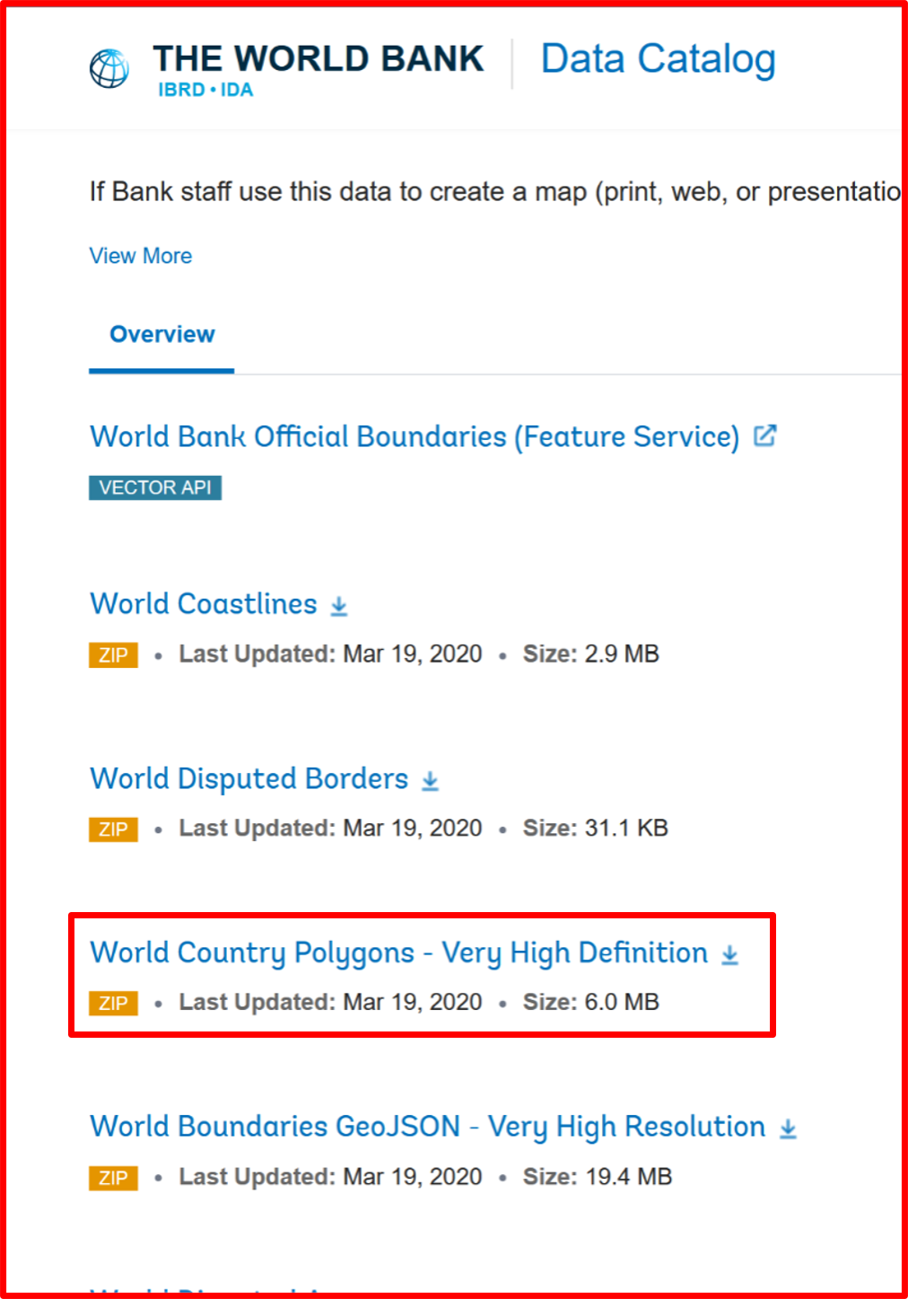
Fig. 4.4.1 Downloading the coutries borders layer
Egypt’s water surfaces from “Freshwater Ecosystems Explorer” for the years 2014 and 2018 (Fig. 4.4.2), in which we can find a layer with one band with three possible values:
1 - Not Water;
2 - Seasonal Water;
3 - Permanent Water.
After downloading the file remember to unzip it before working on it.
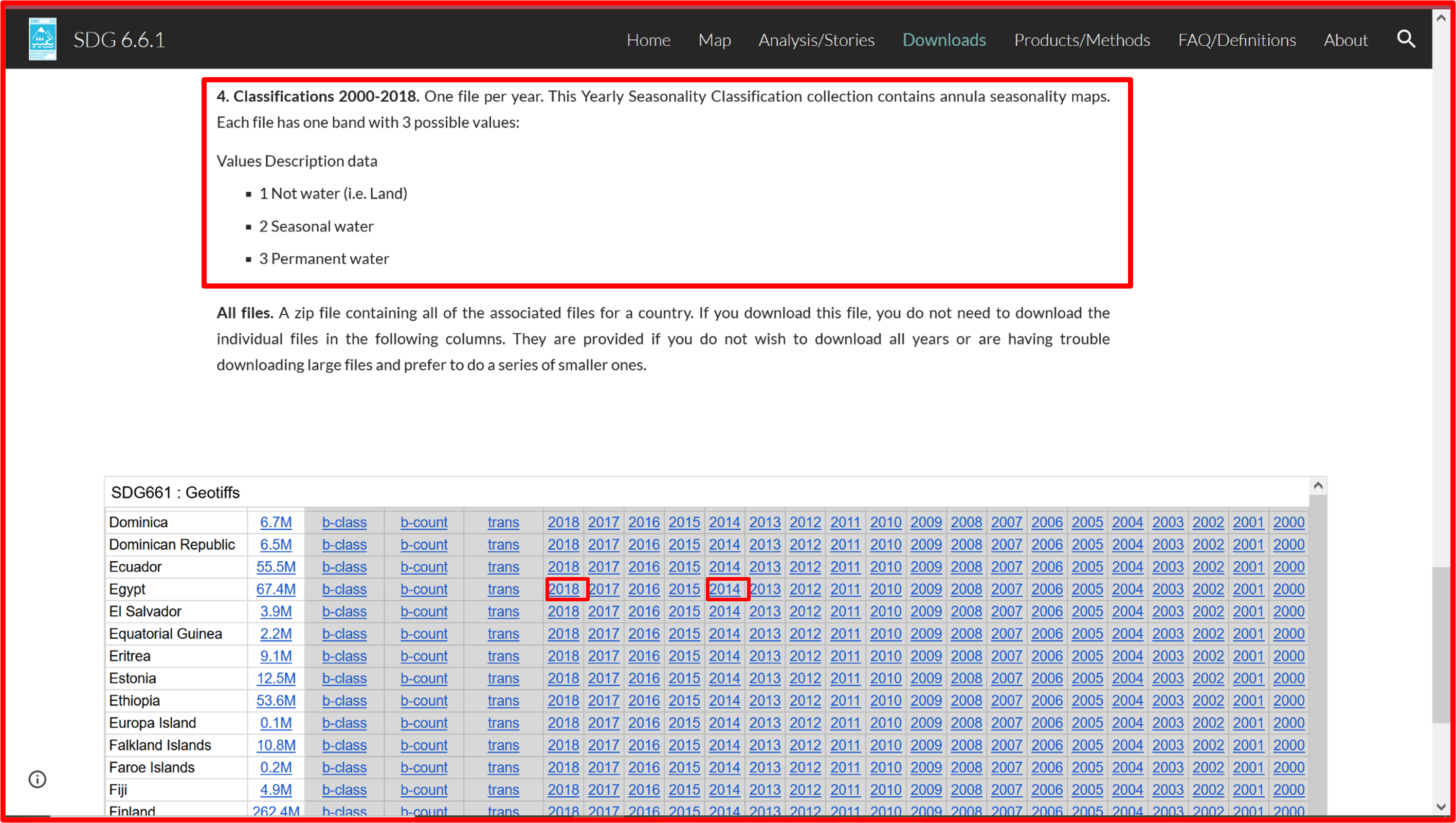
Fig. 4.4.2 Downloading the Egypt’s water surfaces layers
Open a new QGIS project and add the countries borders vector layer to it as in Fig. 4.4.3.
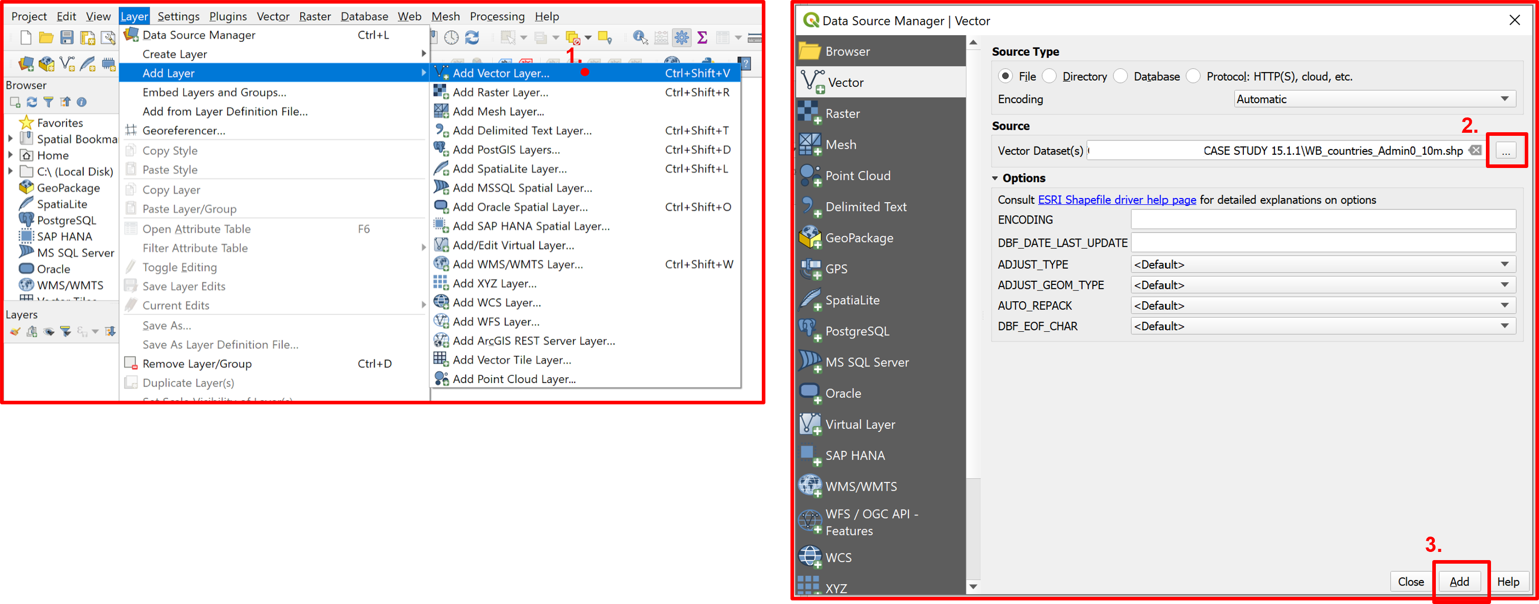
Fig. 4.4.3 Adding the vector layer to the QGIS project
Since we are interested only in Egypt’s water areas, we need to extract its polygon by first selecting it (Fig. 4.4.4) and then extracting the selected features and saving them in a new layer (Fig. 4.4.5).
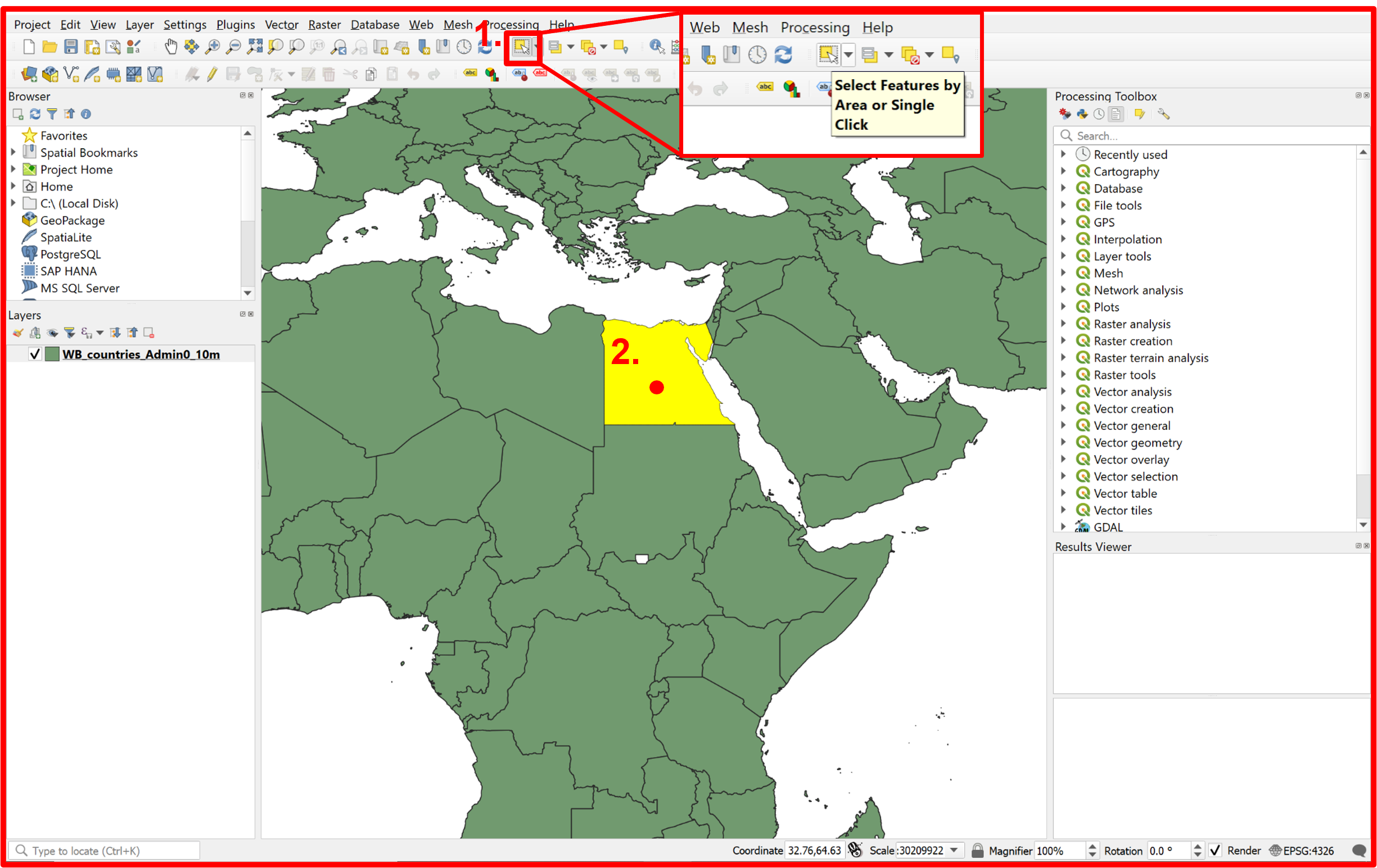
Fig. 4.4.4 Selecting Egypt’s polygon
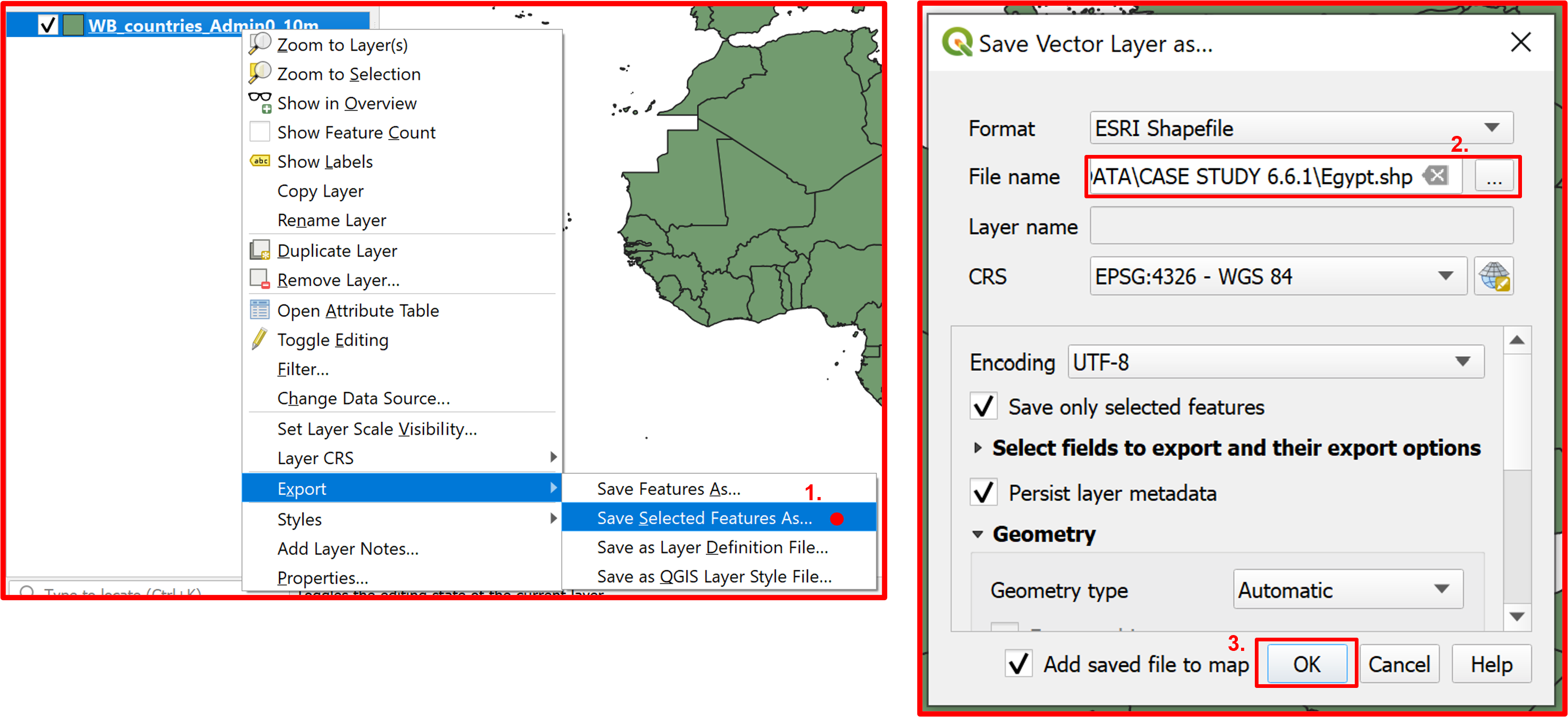
Fig. 4.4.5 Extracting the selected polygon as a new layer
For better visualization purposes change the symbology on the newly added Egypt layer as portrayed in Fig. 4.4.6.
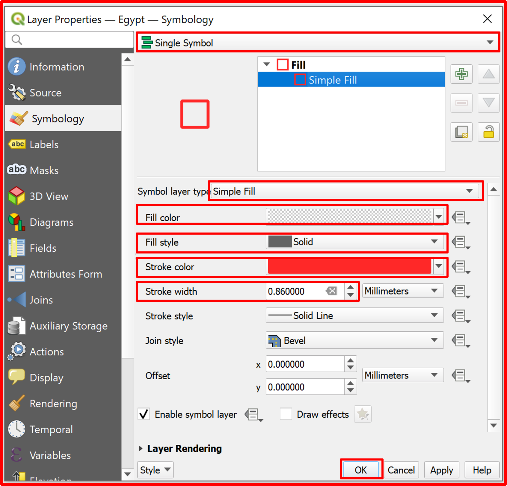
Fig. 4.4.6 Changing the symbology of the “Egypt.shp” layer
Now that we have defined the Area Of Interest (AOI) in our project we can add the water extent data (Fig. 4.4.7).
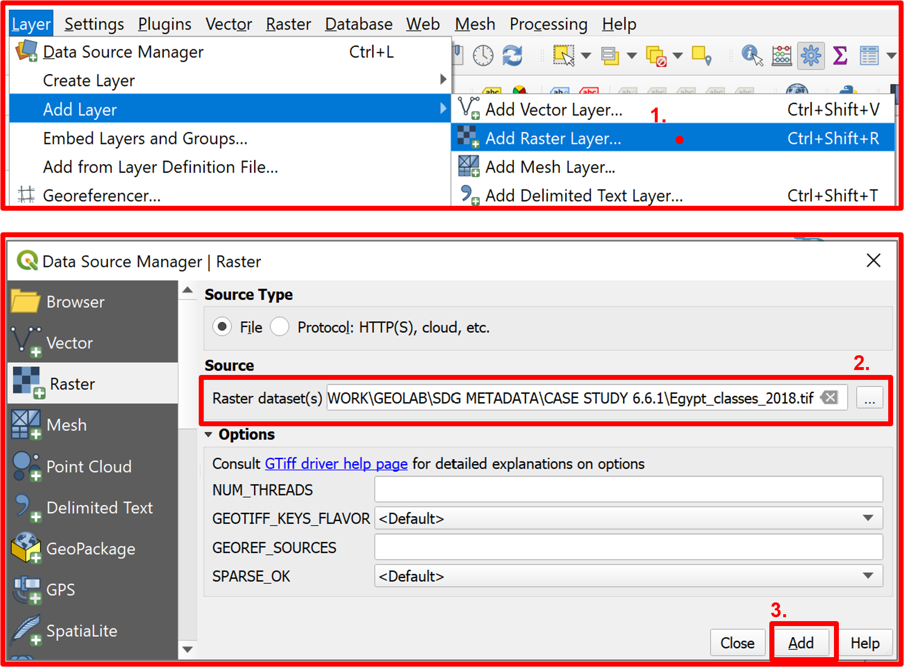
Fig. 4.4.7 Adding the raster layer of the water extent of Egypt in 2018. Repeat for the 2014 layer
As mentioned before each year’s file has three possible values as specified in Fig. 4.4.8, so we want to represent these classes by changing the symbology of both layers. A proposed symbology for the 2018 layer is presented in Fig. 4.4.9. Make sure to apply the symbology change to both layers with the same palette.
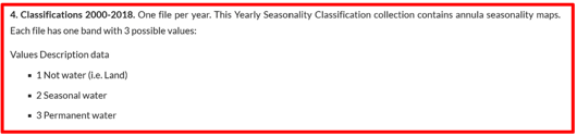
Fig. 4.4.8 Specifications for the raster water extent layers
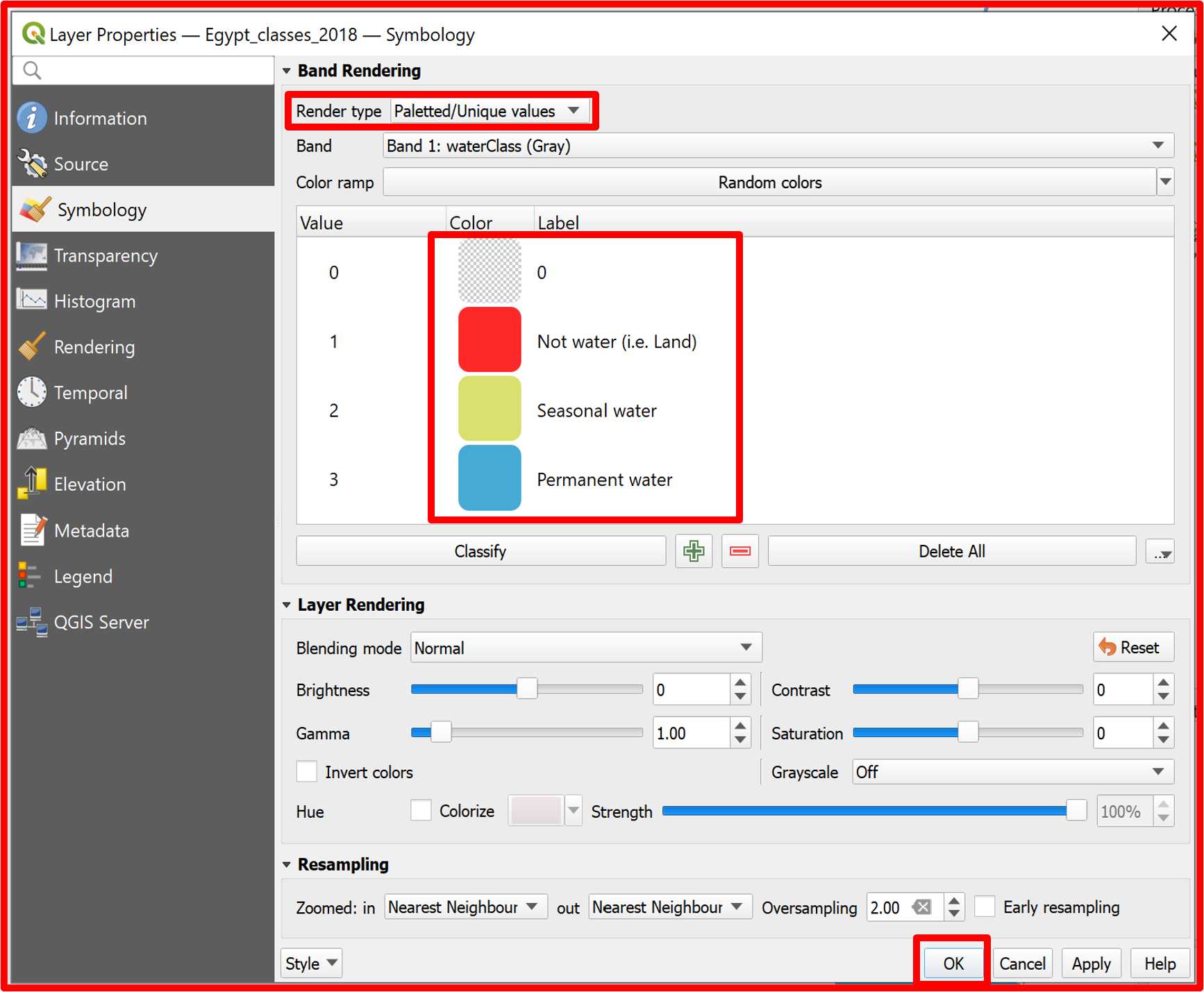
Fig. 4.4.9 Changing the symbology of the water extent layers for better visualization purposes
After adding and changing the symbology of both needed datasets the desired view of the project should be as shown in Fig. 4.4.10.
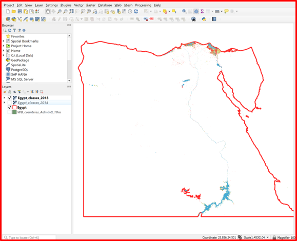
Fig. 4.4.10 The desired view after adding and changing the symbology of the data
Now we need to extract from the two raster layers the components α, β, ρ, σ, ε to calculate the change index as defined in Fig. 4.4.11.
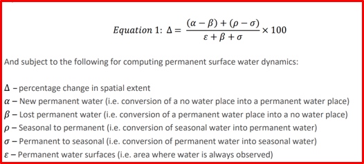
Fig. 4.4.11 The formula of the index to be calculated in this exercise
To do so we will use the “Raster calculator” to create a new raster layer with new values (α, β, ρ, σ, ε) by applying a reclassification scheme presented in Fig. 4.4.12, remembering that the values of the rasters are: 1 - Not Water; 2 - Seasonal Water; 3 - Permanent Water.
The expression “Egypt_classes_2014@1 = 1 AND Egypt_classes_2018@1 = 3” represents the change from a no water place to a water place, which corresponds to α in the equation defined above. After clicking “Run” the process may take a while to complete.
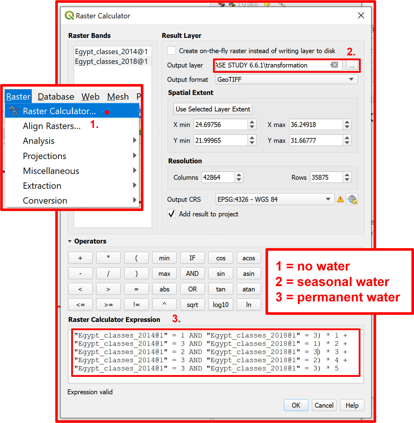
Fig. 4.4.12 Creating a new raster layer with reclassified values according to the needed information for the index calculation
After the process is done the values of the new raster layer will be: * 1 → α; * 2 → β; * 3 → ρ; * 4 → σ; * 5 → ε.
For better visualization change the symbology of the new raster as shown in Fig. 4.4.13.
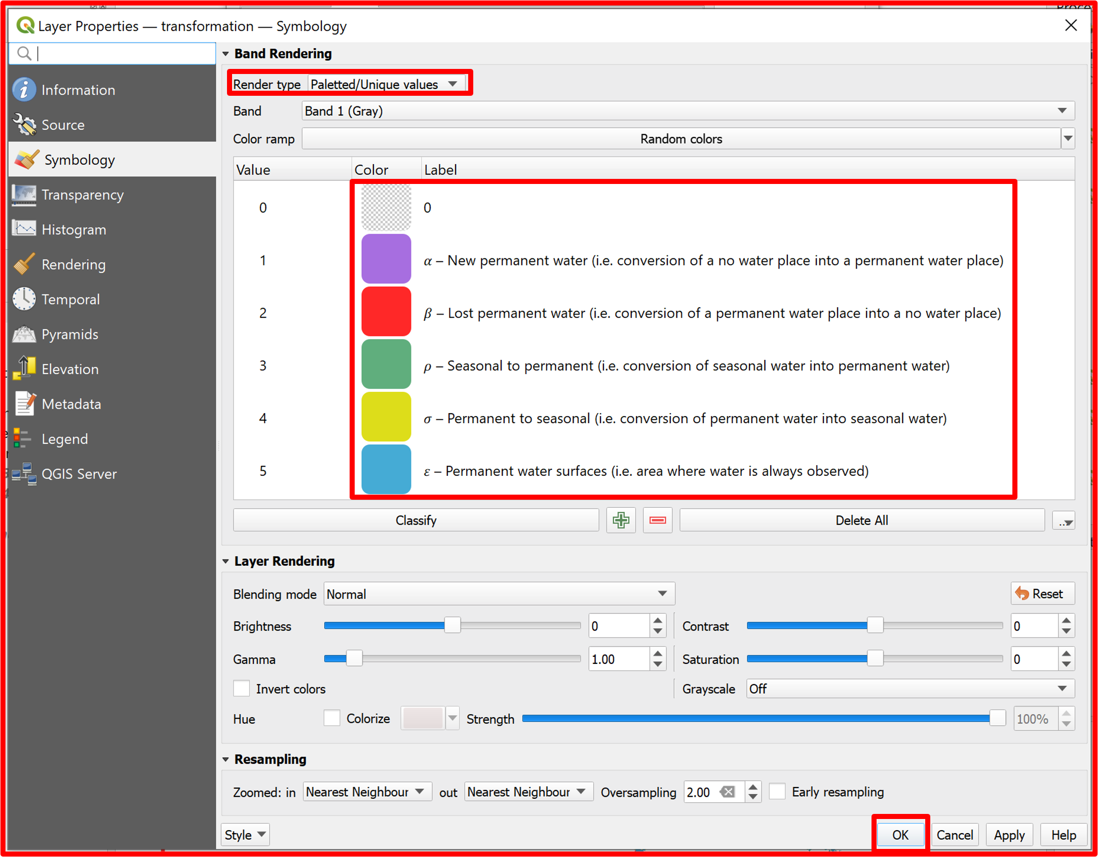
Fig. 4.4.13 Changing the symbology of the new raster
Now that we have a raster showing the changes in permanent water extent we want to know what is their area. To do so we chose the approach of vectorizing the transformation layer for easier computations later on. The process of transforming tre transformation raster layer into a vector layer is heavy and will take a considerable amount of time (YOU CAN DOWNLOAD THE ALREADY VECTORIZED LAYER FROM THE WEBBOOK ZENODO FOLDER). To compute the vector layer we use the “Polygonize (Raster to Vector)” tool from the conversion raster tools (Fig. 4.4.14).
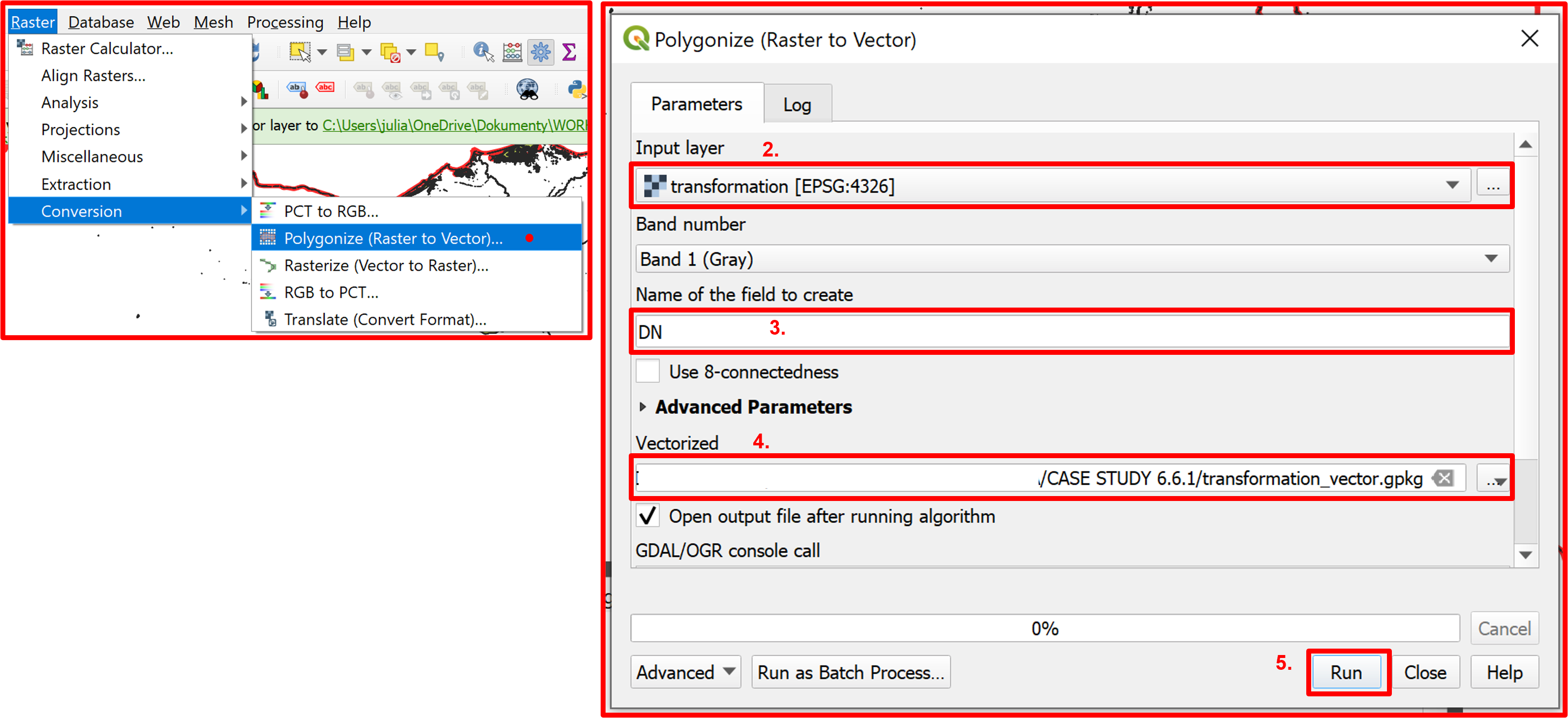
Fig. 4.4.14 Polygonizing the transformation raster
This vector layer also contains land features that we are not interested in, hence we will extract all the features with values not equal to 0. This will be done by first selecting all such features by expression and then exporting the selected features to a new layer. The workflow is presented in Fig. 4.4.15.
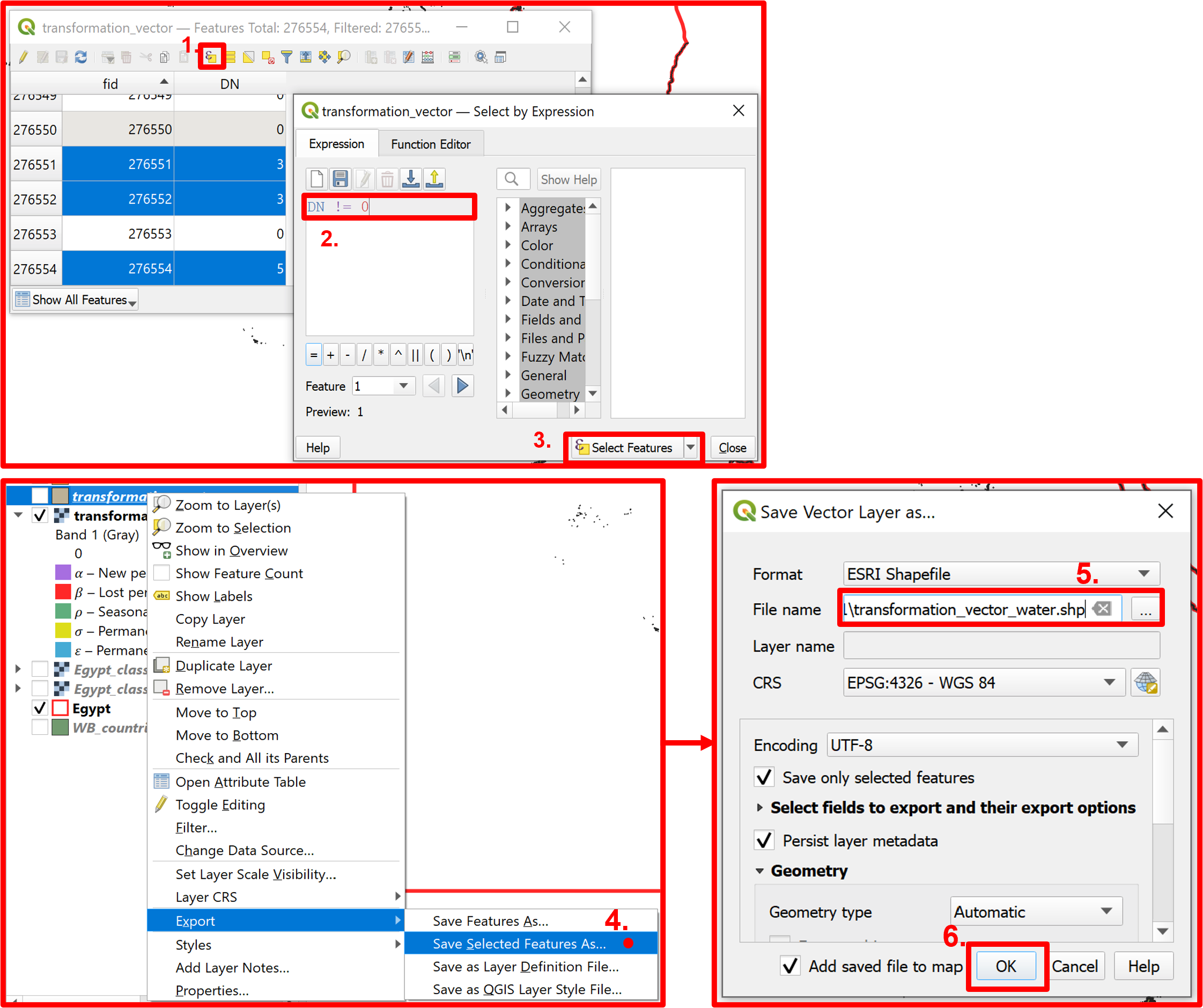
Fig. 4.4.15 Extracting only the information about water areas from the vector
The layer’s attribute table contains all the polygons as separate. We want to group them by their classification so that the attribute table will contain just five classes representing the component of the final equation. To do that we will use the “Dissolve” geoprocessing tool. It is important to remember what is the field that we are dissolving and set it in the optional settings of the process. The procedure is presented in Fig. 4.4.16.
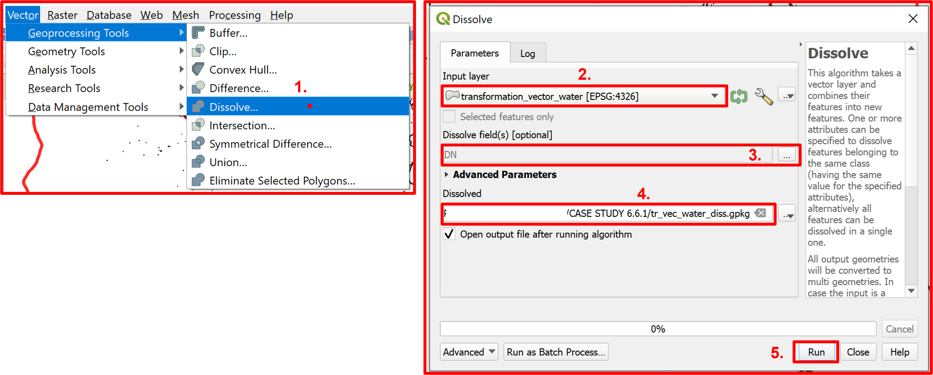
Fig. 4.4.16 Dissolving the features of the vector according to the class field (DN)
Now that we have all of our component’s classes grouped we can calculate each class’ area to have the final values for the computation. We will use the “Add Geometry Attributes” vector geometry tool using as input the dissolved transformation vector containing water information. The ellipsoidal parameter should be set in the calculation parameter (Fig. 4.4.17).
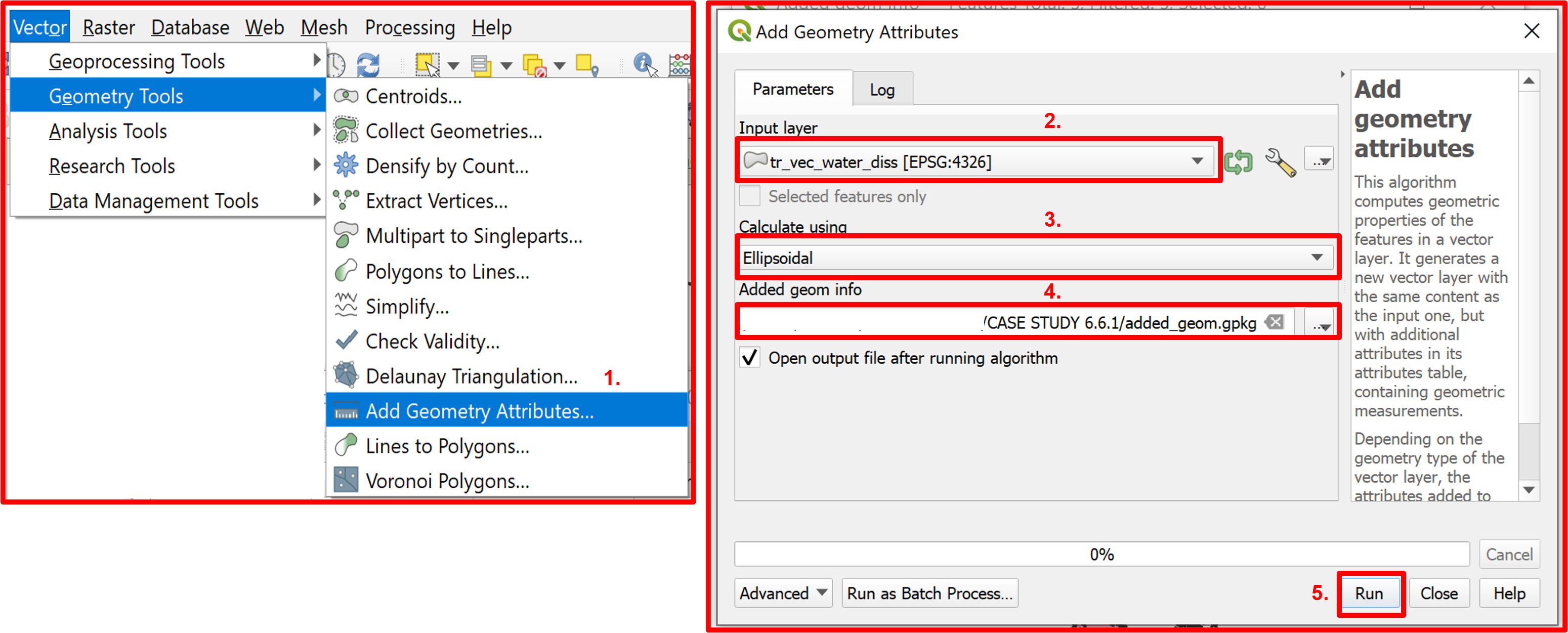
Fig. 4.4.17 Adding geometry attributes to the vector layer
The output vector layer will now contain the area for each type of water transformation (Fig. 4.4.18).
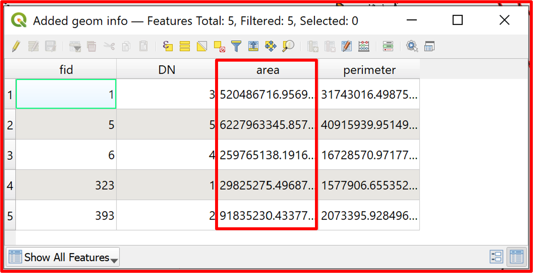
Fig. 4.4.18 The final view of the attribute table of the vector layer
The values can be plugged in directly to the equation to get the final result of the exercise as the percentage change in spatial extent of permanent water. Remember that in our case: 1 → α; 2 → β; 3 → ρ; 4 → σ; 5 → ε. The area change of permanent water component of the SDG indicator 6.6.1 is equal to approximately 3%, which indicates that in the 2014-2018 period there was an increase (because it’s positive) of permanent water areas of 3%.