4.2. Ratio of land consumption rate to population growth rate [11.3.1]

In this section you will learn how to calculate the SDG indicator 11.3.1 which is defined as the ratio of land consumption rate to population growth rate. To be able to derive this indicator we need to first define the population growth and the land consumption rate.

The population growth rate (PGR) is the change of a population in a defined area during a period, expressed as the percentage of the population at the start of that period. Its value depends on the number of births and deaths and on the migration patterns in the given period. In SDG 11.3.1 the PGR is computed for city areas. The land consumption rate (LCR) is defined as the rate at which urbanized land changes through a defined period of time. The LCR is expressed as the percent of the land occupied by the city/urban area at the start of that time. SDG 11.3.defines “land consumption” as the conversion of land from non-urban to urban functions. For the correct calculation of the index it is also needed to agree on what constitutes a city or urban area. For this purpose we will be using the Degree of Urbanization (DEGURBA) method to delineate cities, urban and rural areas for international statistical comparisons endorsed by the United Nations Statistical Commission For more information about the background of the SDG indicator 11.3.1 read the metadata provided under this link The workflow for computing the indicator follows 5 steps:

1. Decide on the analysis period

2. Delimitation of the urban area which we will analyze

3. Computation of the land consumption rate

4. Computation of the population growth rate

5. Computation of the ratio of LCR to PGR

1. In this exercise we will work on a one year interval from 2018 to 2019.

2. We will use New Delhi as the analysis area. Download from https://ghsl.jrc.ec.europa.eu/ghs_stat_ucdb2015mt_r2019a.php the delimitation of urban areas file as shown in (Fig. 4.2.1).

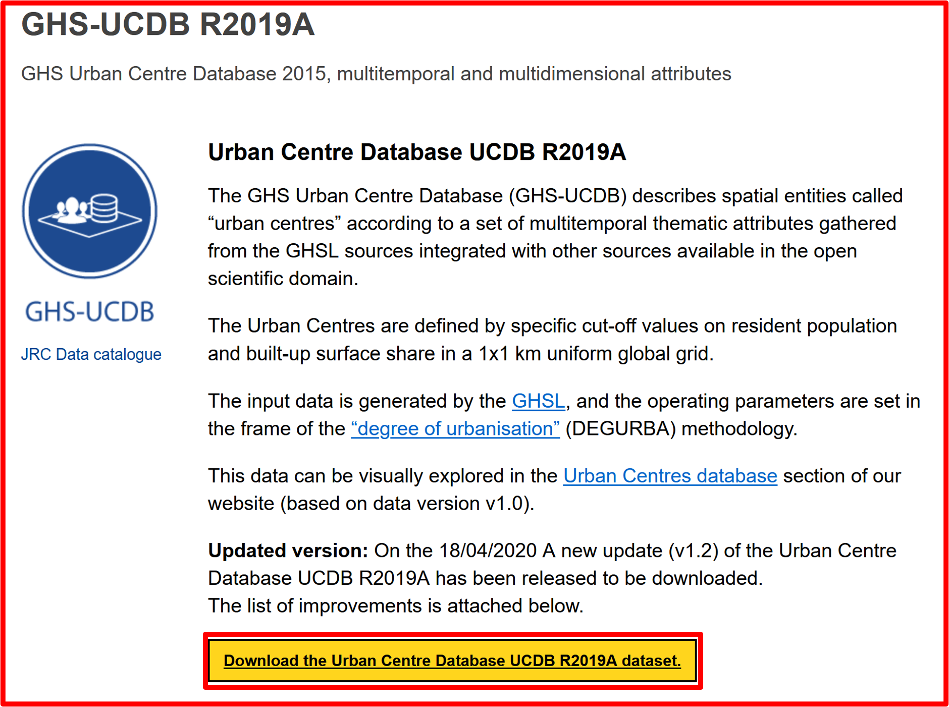
Fig. 4.2.1 Downloading the delimitation of urban areas file

Open a new QGIS project and add the downloaded vector (.gpkg) file to it (Fig. 4.2.2).

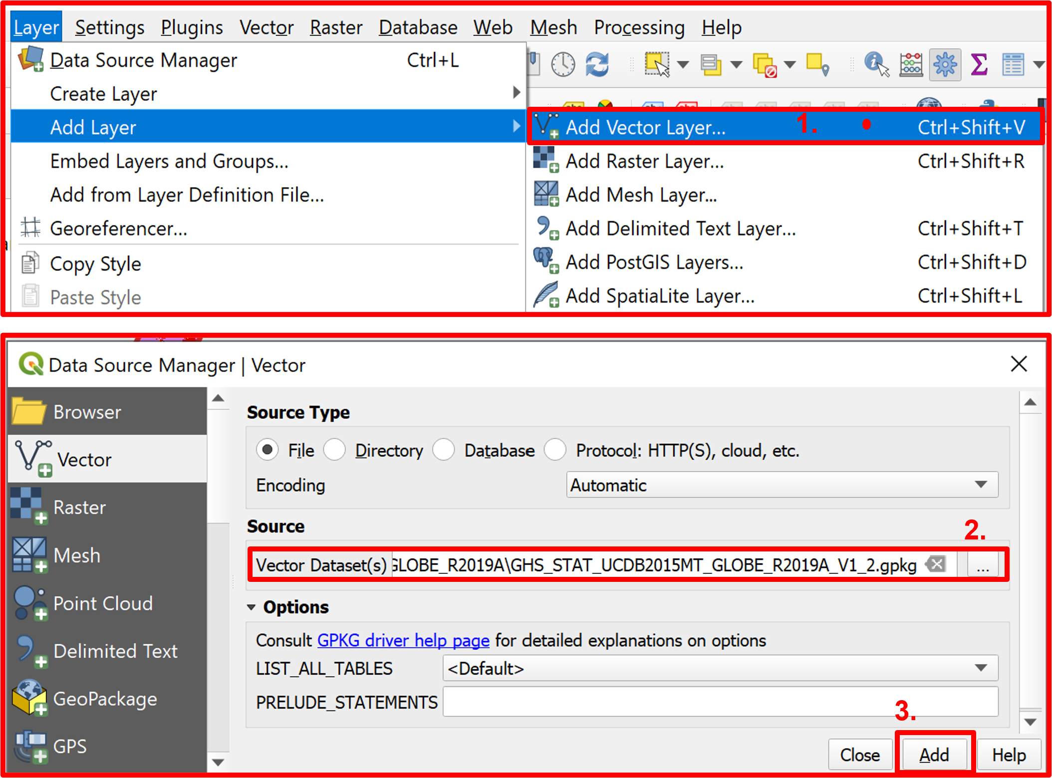
Fig. 4.2.2 Adding the vector layer to a new QGIS project

We now want to extract only the delineation of New Delhi. After opening the attribute table of the just added layer, click on the “Select features using an expression” icon (Fig. 4.2.3).

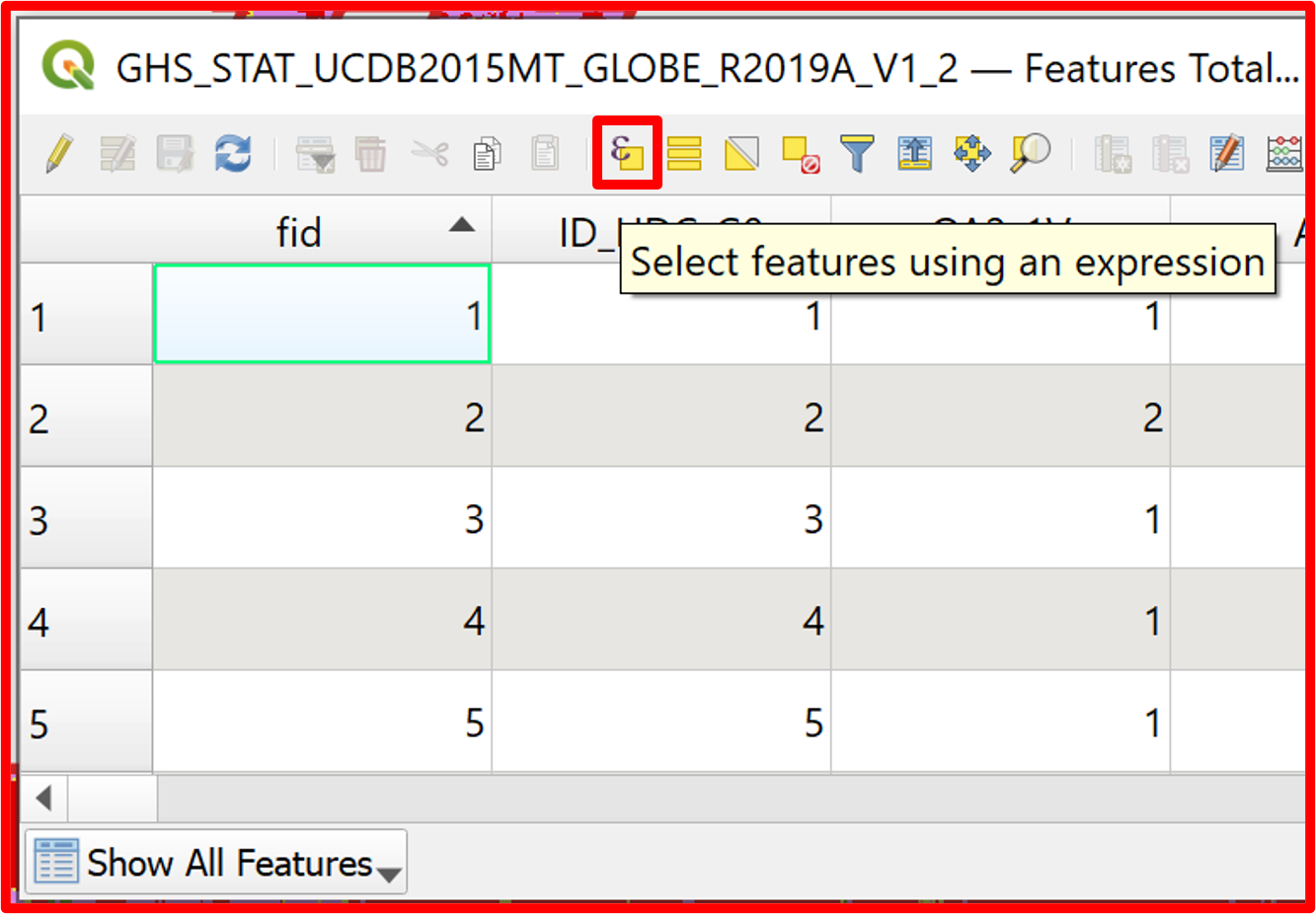
Fig. 4.2.3 Select features using an expression button in the attribute table

After the Selection by Expression window appears, enter the query: UC_NM_MN = "Delhi [New Delhi]" and click on “Select Features” (Fig. 4.2.4).

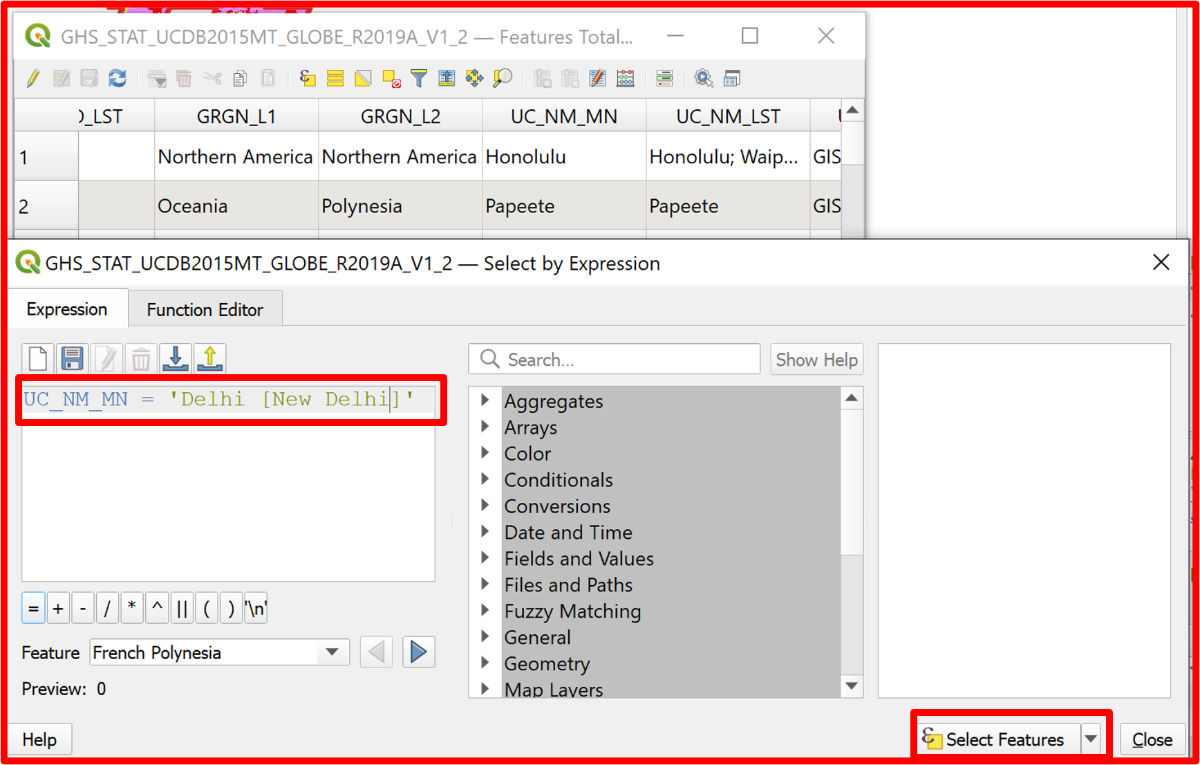
Fig. 4.2.4 Selecting features by expression

After selecting New Delhi, extract it to a new vector layer “NewDelhi.shp” as shown in Fig. 4.2.5.

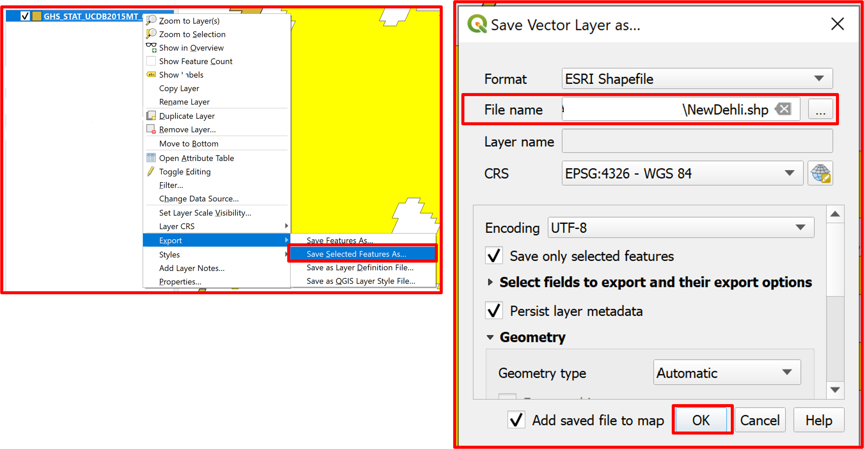
Fig. 4.2.5 Saving selected features as new vector layer

Change the symbology of the “NewDelhi.shp” layer to better visualize the delineation of the urban area (Fig. 4.2.6).

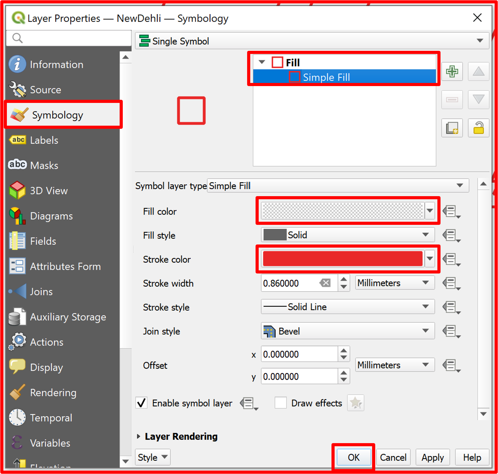
Fig. 4.2.6 Symbology of the New Delhi shapefile vector layer

3. To compute the land consumption rate in the period 2018-2019 we need the urban areas data from both of the year. We can access the Land Cover raster data from https://lcviewer.vito.be/download. Download the indicated tile from 2018 and 2019 as shown in Fig. 4.2.7.

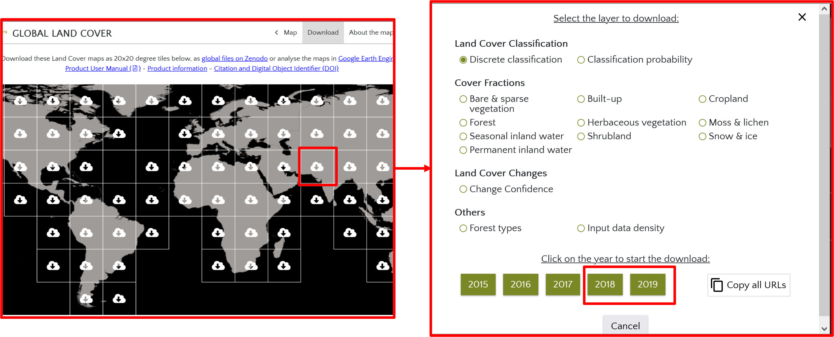
Fig. 4.2.7 Land cover raster data download

After downloading both raster layers, add them to your QGIS project (Fig. 4.2.8).

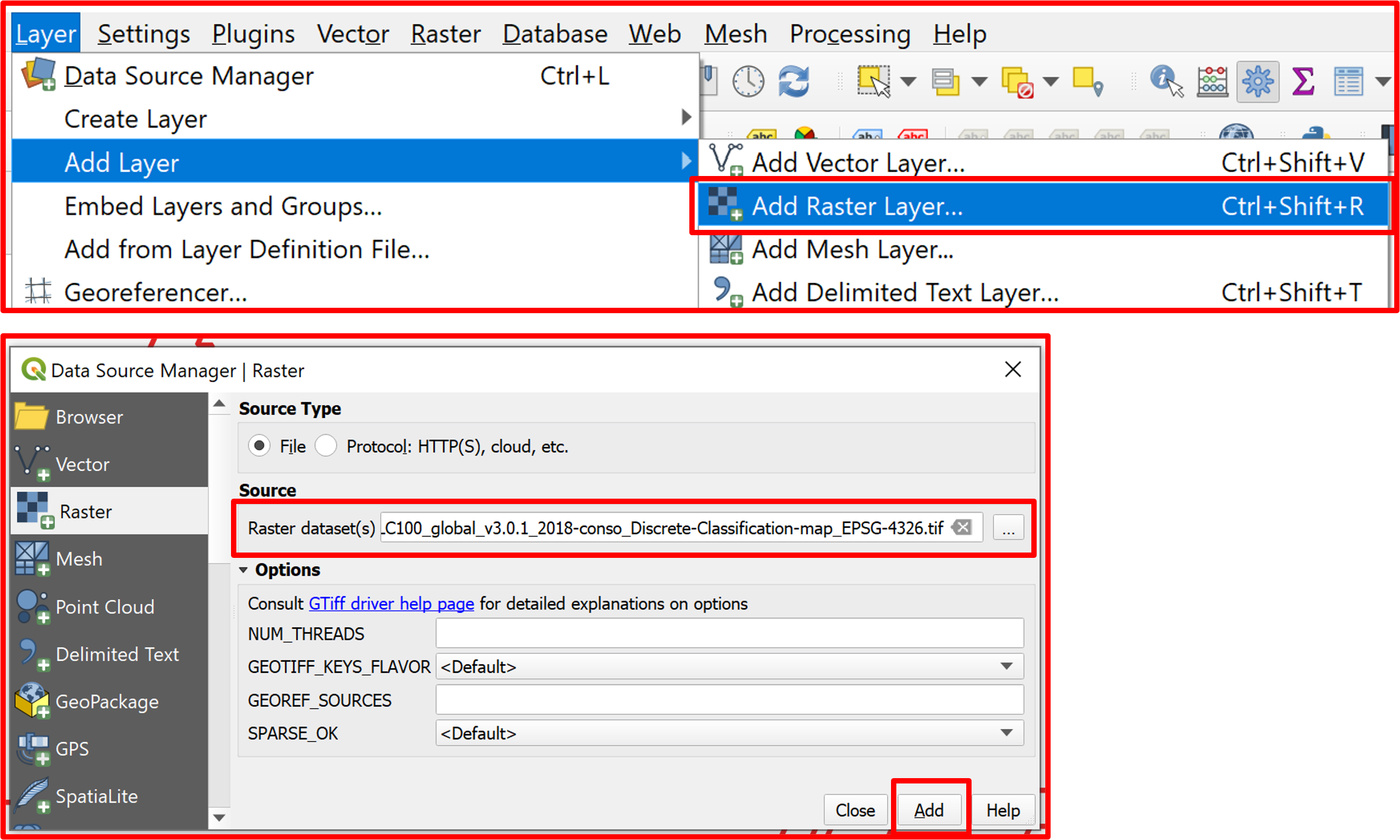
Fig. 4.2.8 Adding the raster layers into the QGIS project (repeat for the 2019 layer)

Now, clip both layers by mask of the New Delhi boundary, so that we will work only on the area of interest (Fig. 4.2.9).

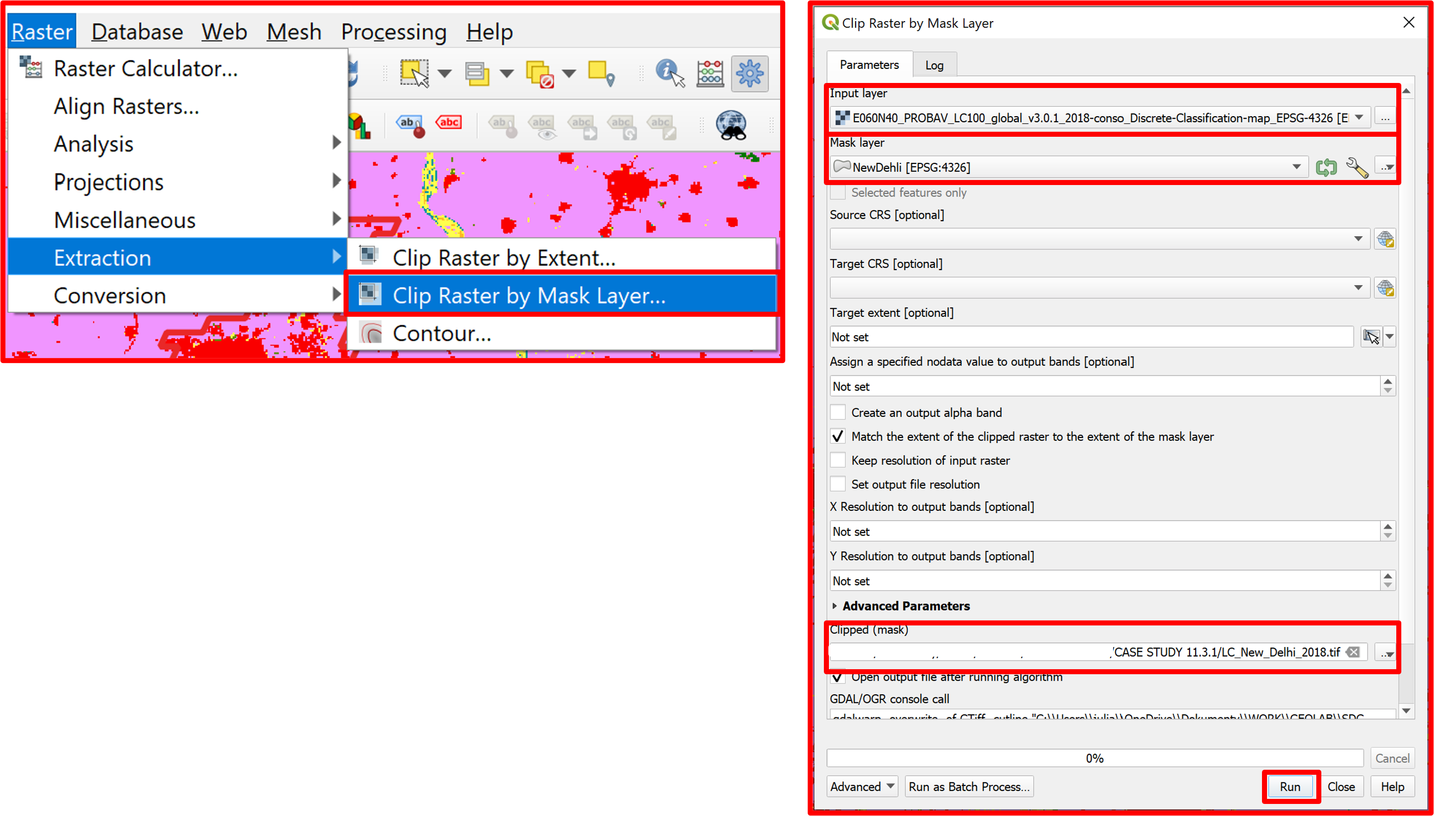
Fig. 4.2.9 Clipping the raster layer by the New Delhi boundary mask (repeat for the 2019 layer)

Since we need only the urban areas of New Delhi, we would like to extract from the layers only the pixels representing urban/built up areas. From the Copernicus Global Land Service: Land Cover 100m: version 3 Globe 2015-2019: Product User Manual we know that the map code for the urban/built up class is 50 (Fig. 4.2.10).

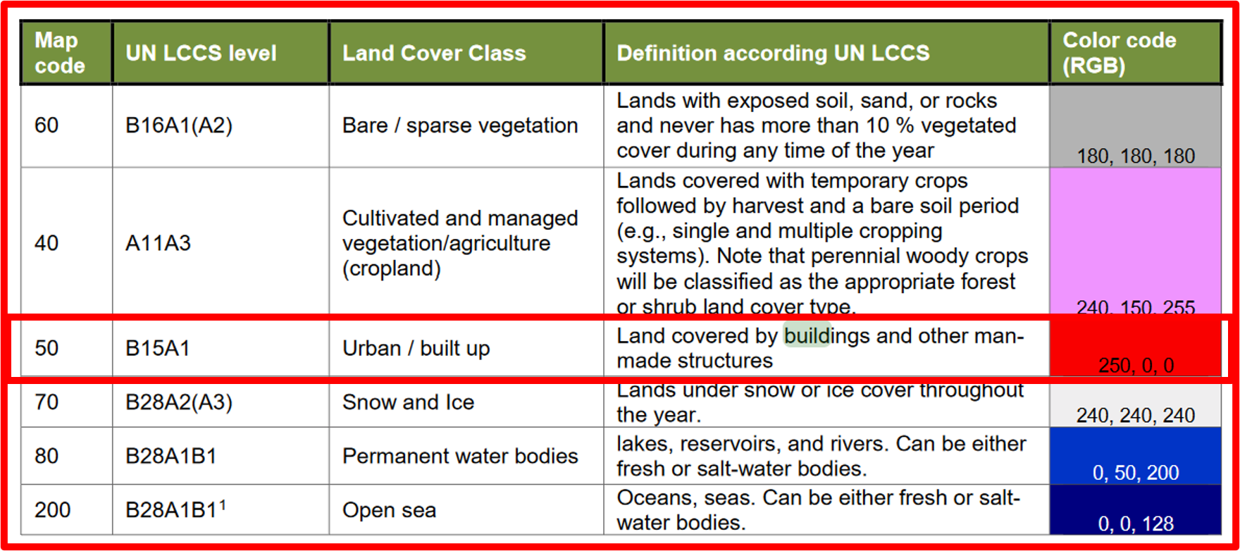
Fig. 4.2.10 Classification of the land cover layer with map codes

We need to reclassify both rasters so that the pixels with the value of 50 have the value of 1 and the rest the value of 0. This step is performed by using the “Raster Calculator” and inputting the expression: (“LC_New_Delhi201x@1” = 50) * 1 + (“LC_New_Delhi201x@1” != 50) * 0, where x is equal to 8 or 9 depending on the layer. The procedure for the 2018 layer is shown in Fig. 4.2.11.

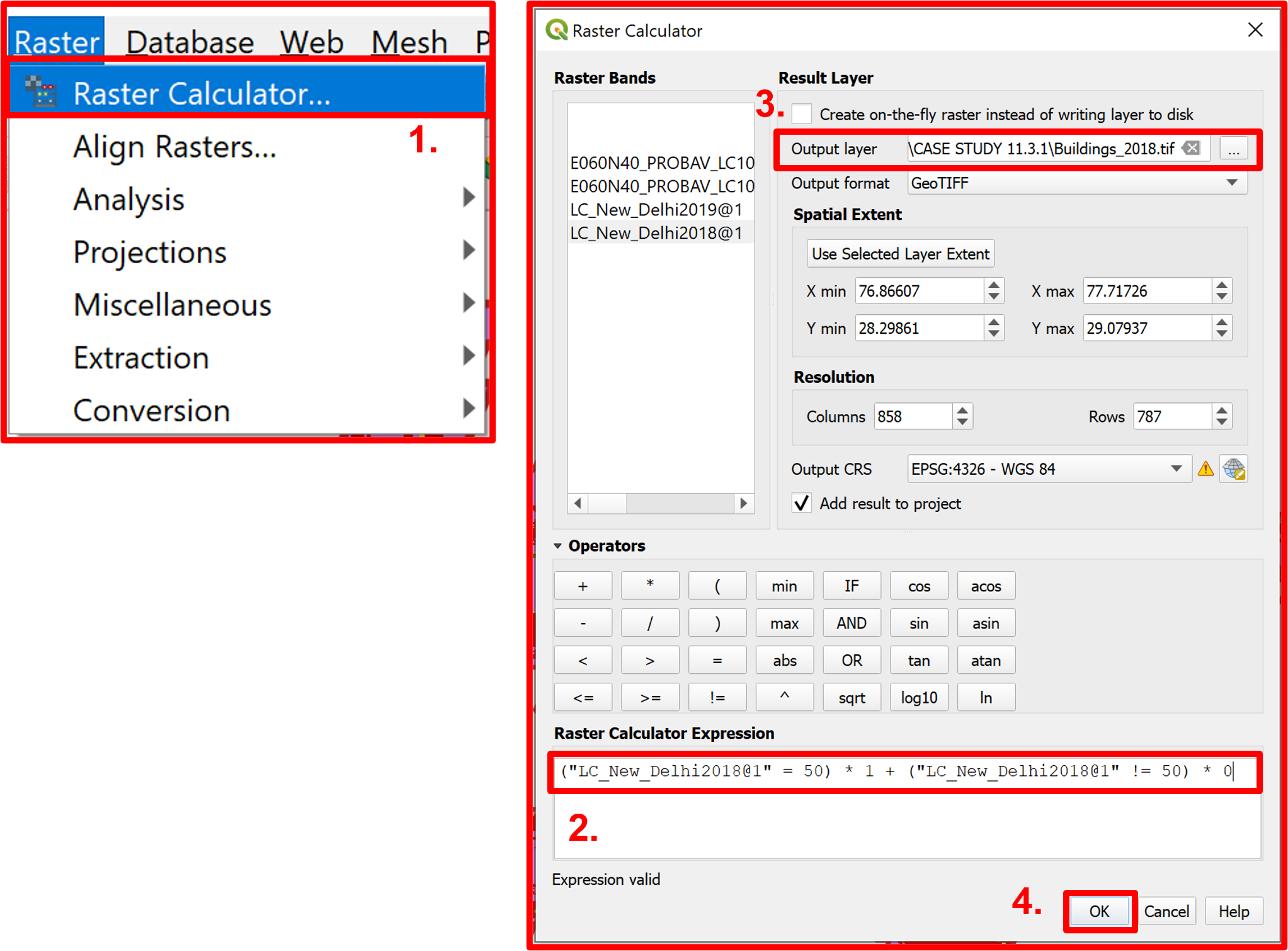
Fig. 4.2.11 Raster reclassification (repeat for the 2019 layer)

For better visualization, change the symbology of both reclassified layers, so that the render type is set to “Paletted/Unique values” and the color of class 0 is set to transparent, as shown in Fig. 4.2.12.

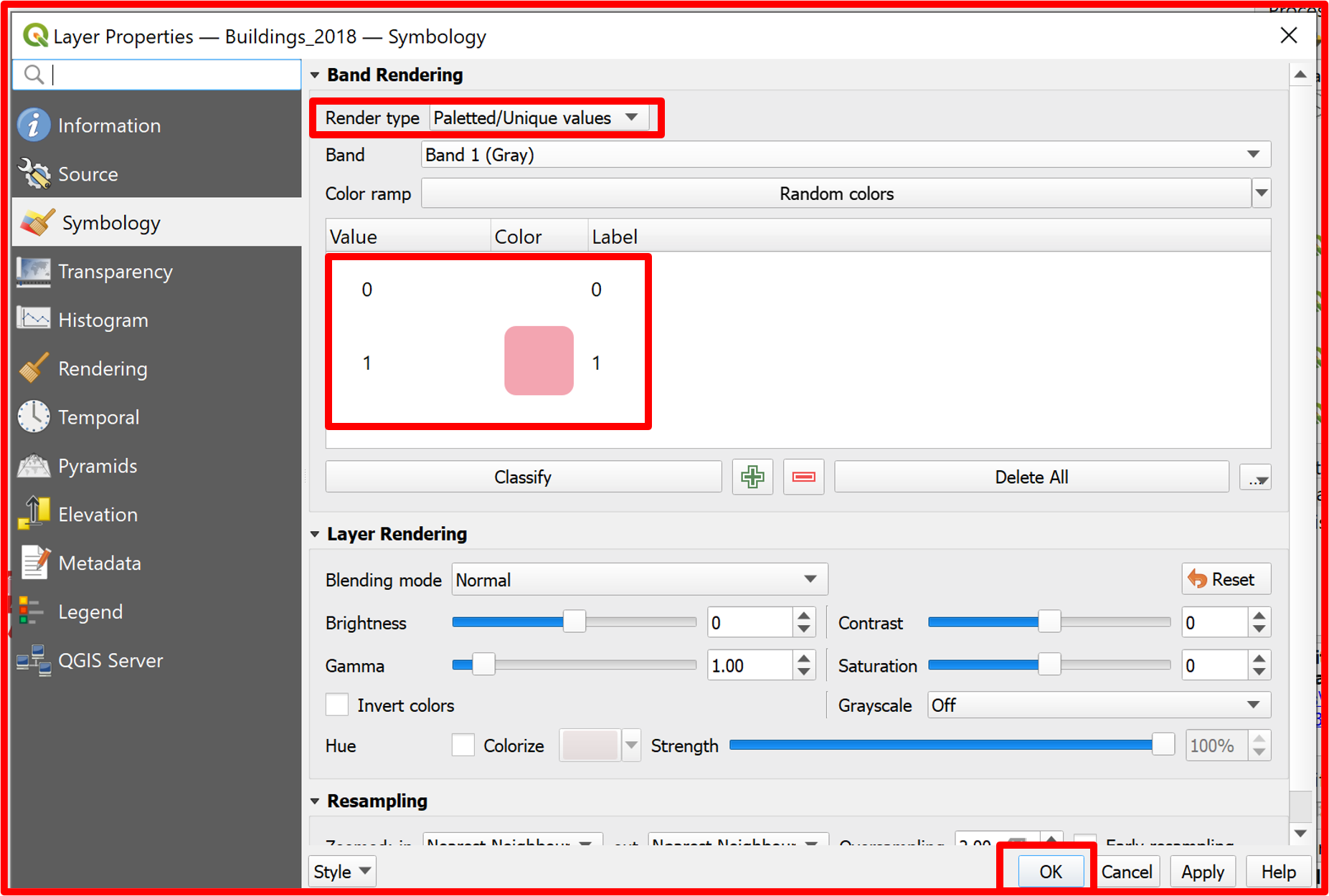
Fig. 4.2.12 Symbology properties for the reclassified land cover raster layers (repeat for the 2019 layer)

The desired view after clipping, reclassifying and changing the symbology of the LC layer is as in Fig. 4.2.13.

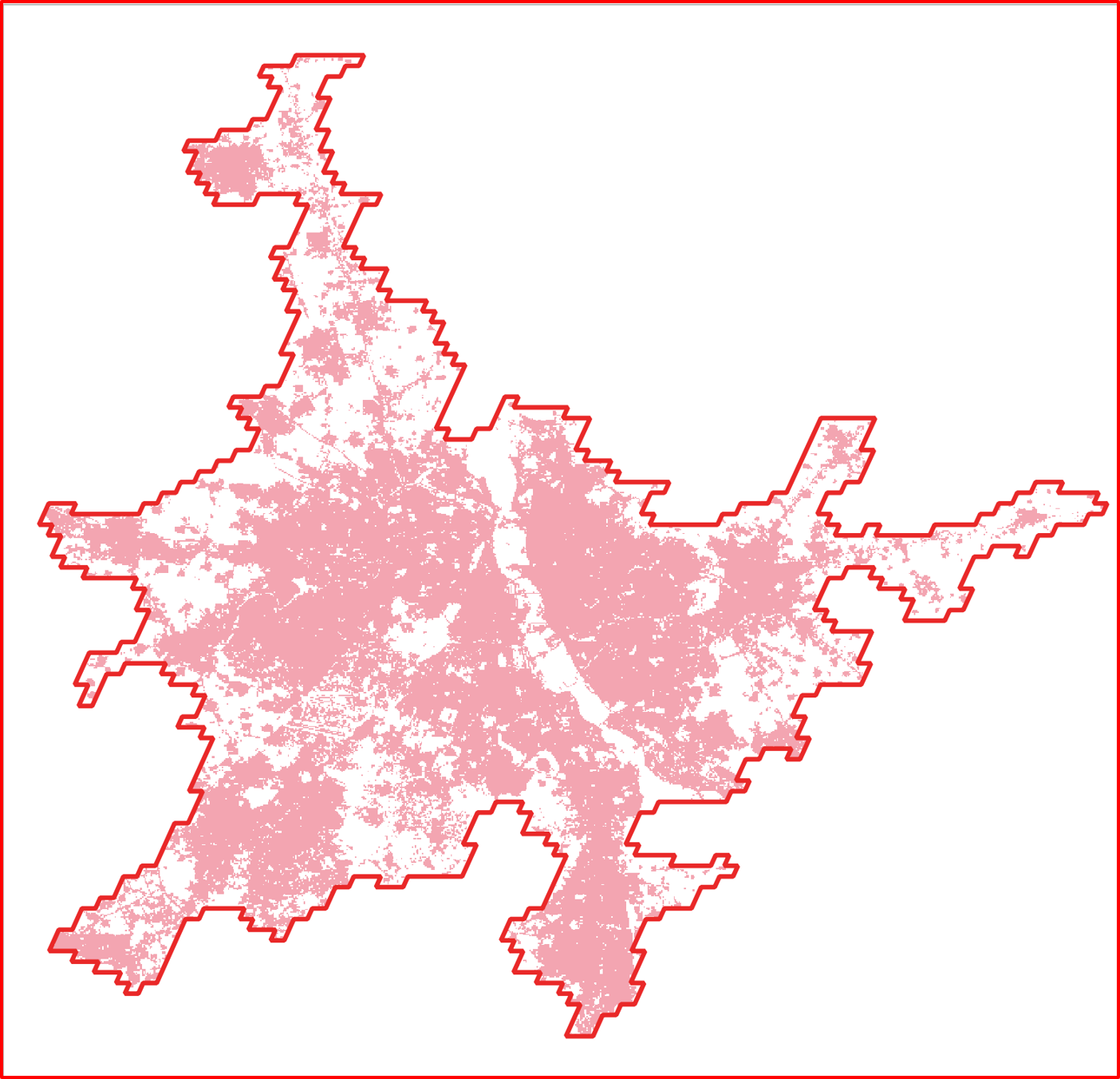
Fig. 4.2.13 Land cover layer of the urban areas after the preprocessing steps

To be able to calculate the Land Consumption Rate, we must know the area of the built up zones in both years. To do so, we firstly calculate the sum of the pixels by using the “Zonal Statistics” tool (Fig. 4.2.14). By calculating the sum of all pixels we will actually get the sum of the pixels representing the urban class, as they have value 1 and the rest has value 0.

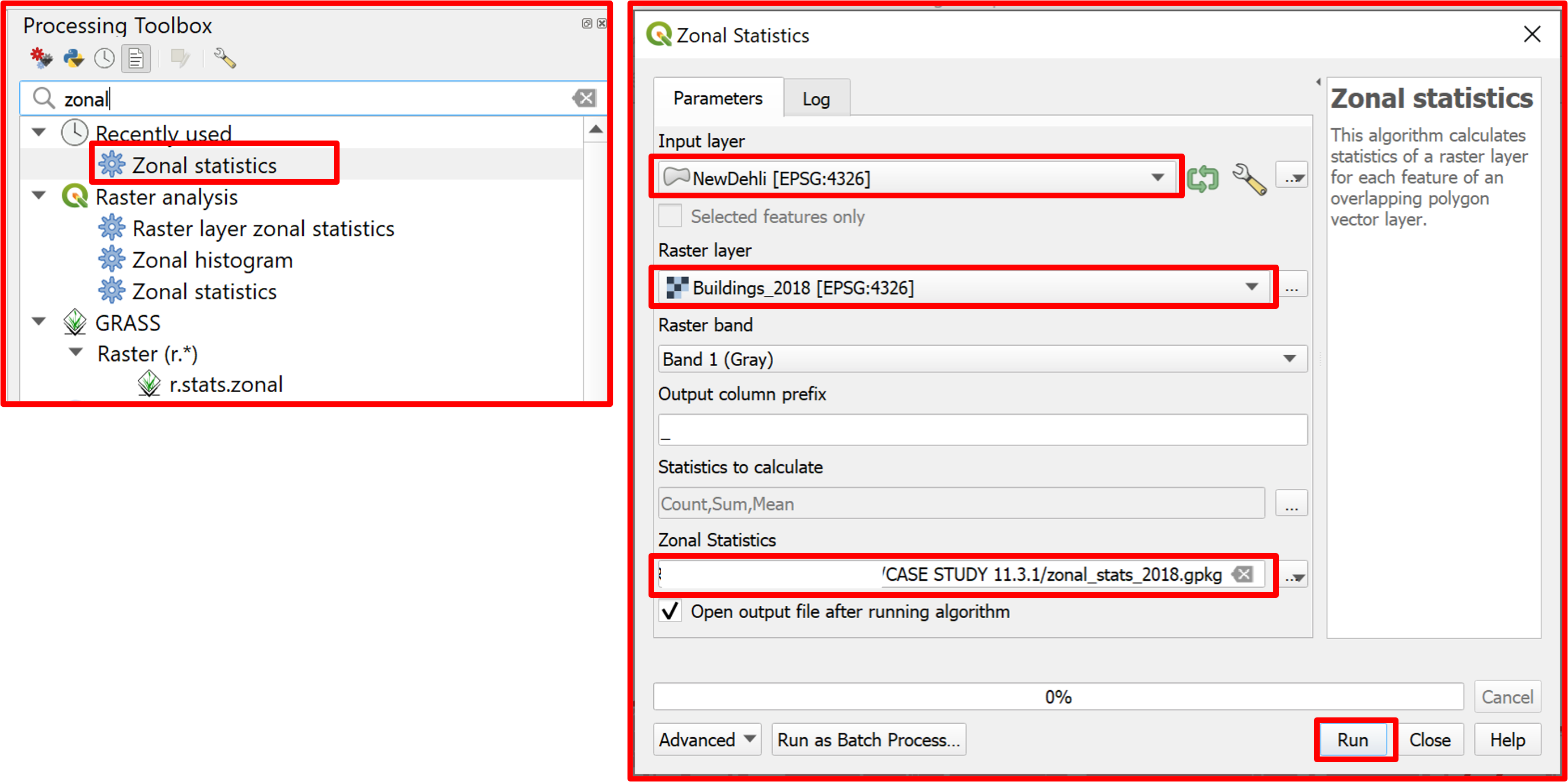
Fig. 4.2.14 Calculating the sum of pixel values using “Zonal statistics”

Having the zonal_stats layers with the sum of the urban pixels, we can now calculate the area of the urban zones in New Delhi in both years, knowing that the pixel size is 100x100m. For both zonal_stats layers open the field calculator and add a new field for the built up area in square km. Calculate the value of the field by multiplying the “_sum” field by 0.1 * 0.1 (km). The step for the “zonal_stats_2018” is shown in Fig. 4.2.15, be sure to repeat the step also for “zonal_stats_2019”.

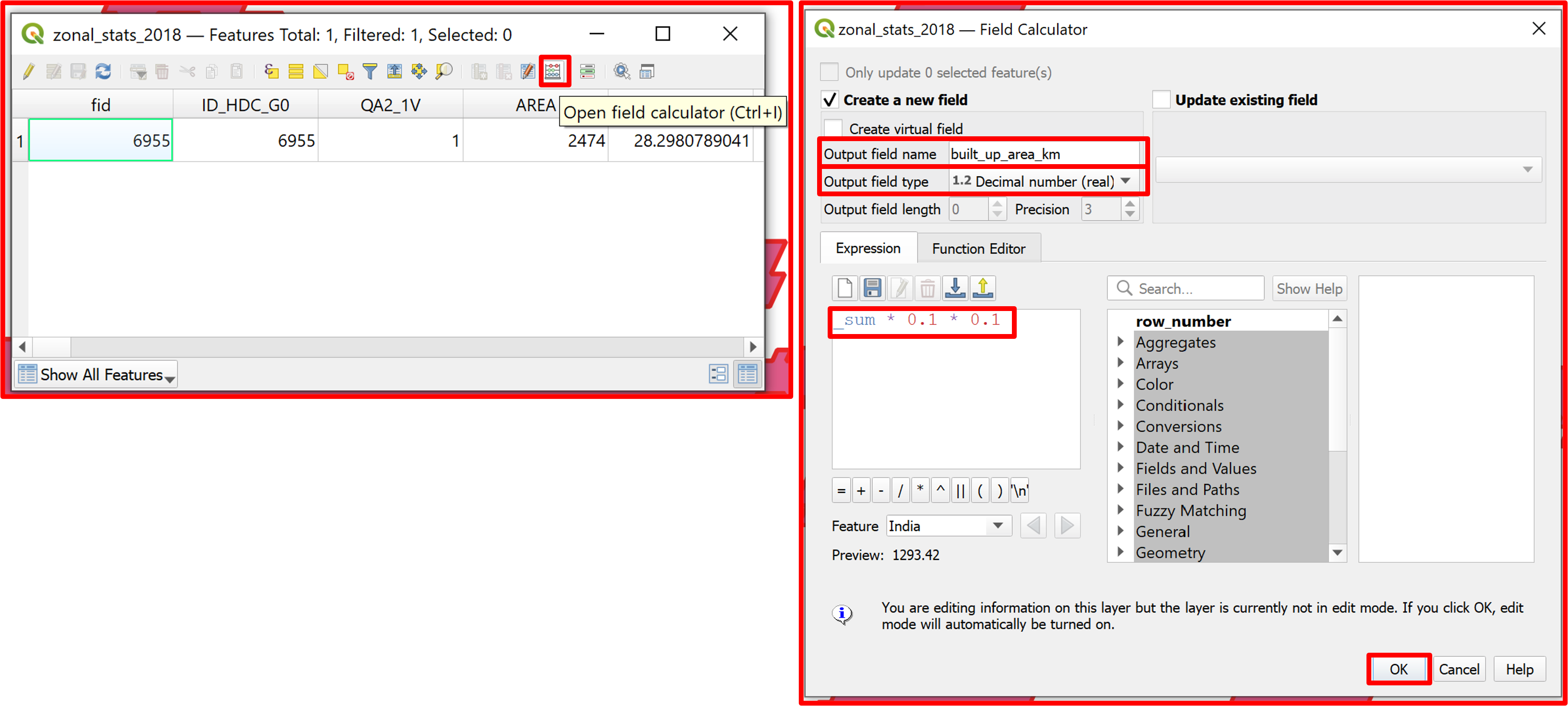
Fig. 4.2.15 Calculating the urban area in square kilometers (repeat for the 2019 layer)

Finally, it is possible to calculate the Land Consumption Rate (LCR) by applying this formula: LCR = (Vpresent - Vpast)/Vpast, to the calculated values in the previous steps. We will calculate it in a new field in the attribute table of the “zonal_stats_2018” layer as shown in Fig. 4.2.16.

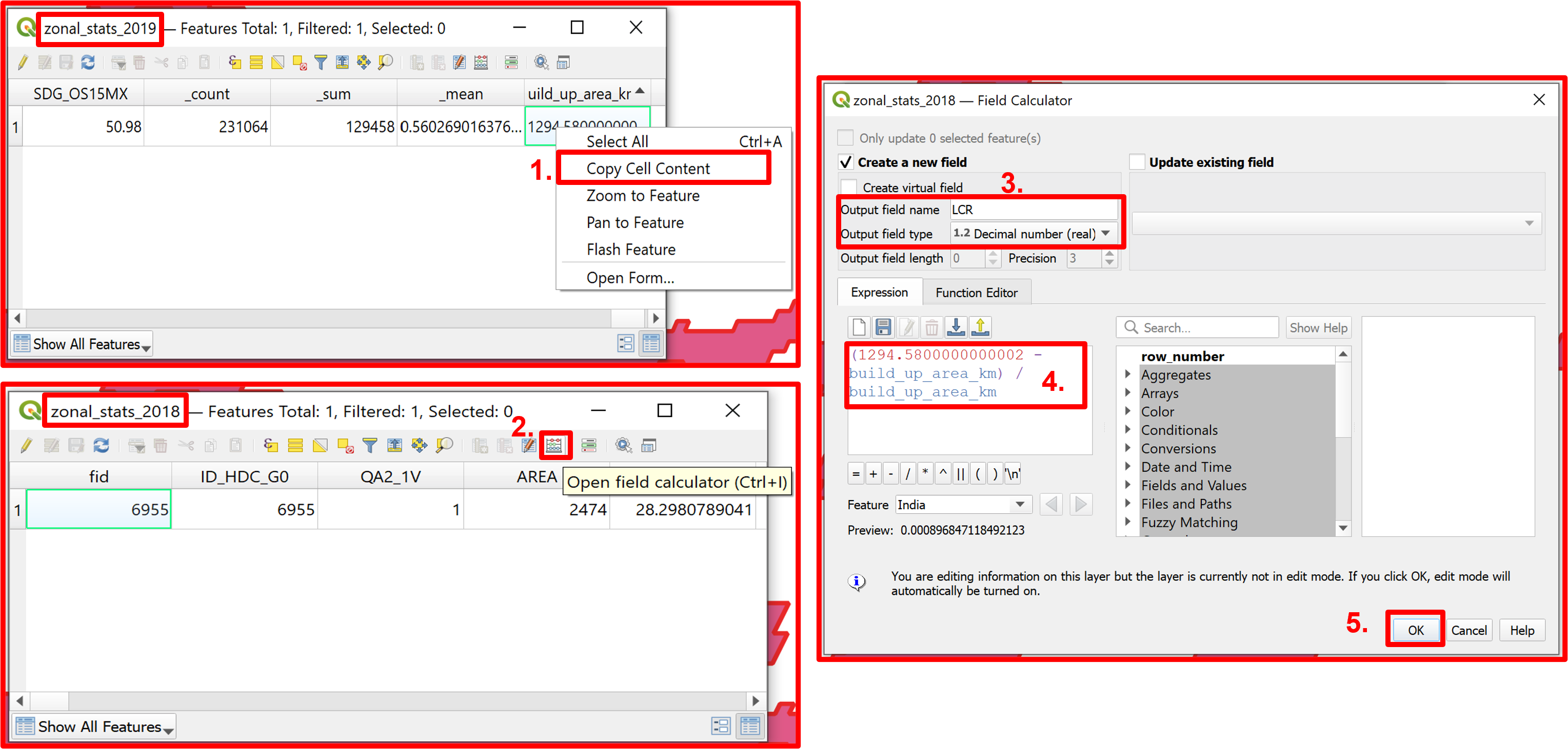
Fig. 4.2.16 Calculating the Land Consumption Rate

4. Having calculated the LCR, it is time to calculate the second index needed to calculate SDG 11.3.1 - the Population Growth Rate.

The PGR is calculated using the total population within the urban area for the analysis period using the formula below:

\(PGR = \frac{\ln(\frac{Pop_{(t+n)}}{Pop_t})}{y}\),

where:

• \(\ln\) is the natural logarithm value;

• \(Pop_t\) is the total population within the urban area in the initial year;

• \(Pop_{t+n}\) is the total population within the urban area in the final year;

• \(y\) is the number of years between the two measurement periods.

Thus, to calculate the PGR we need the population of New Delhi in 2018 and in 2019. To get this information we first need to download the population layers for India in 2018 and 2019 from https://hub.worldpop.org/geodata/listing?id=29 by clicking “Data & Resources” and then “Download Entire Dataset” (Fig. 4.2.17).

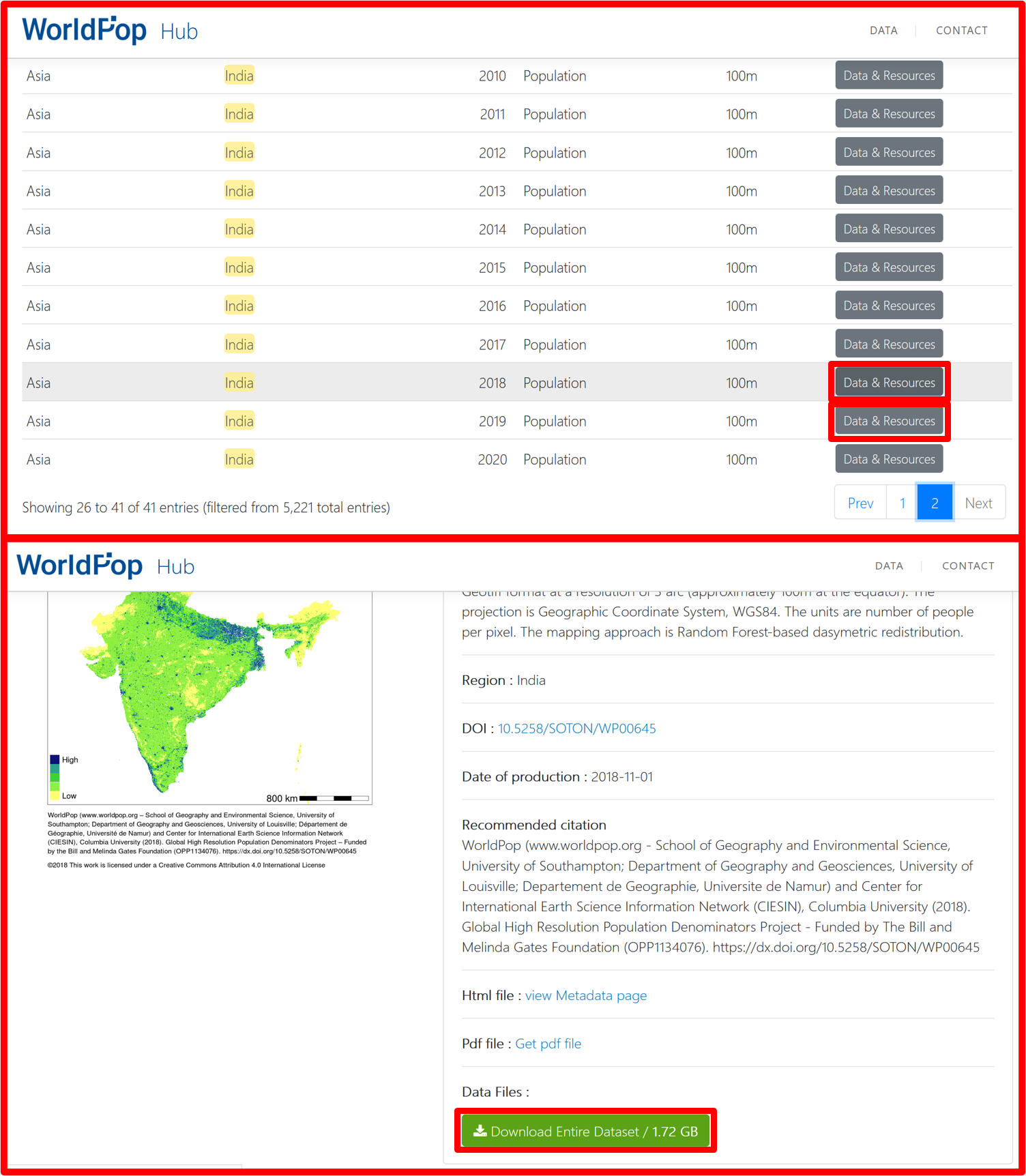
Fig. 4.2.17 Downloading the population layers for India

Load the population layers to the QGIS project and clip them both to New Delhi boundaries. (Fig. 4.2.18).

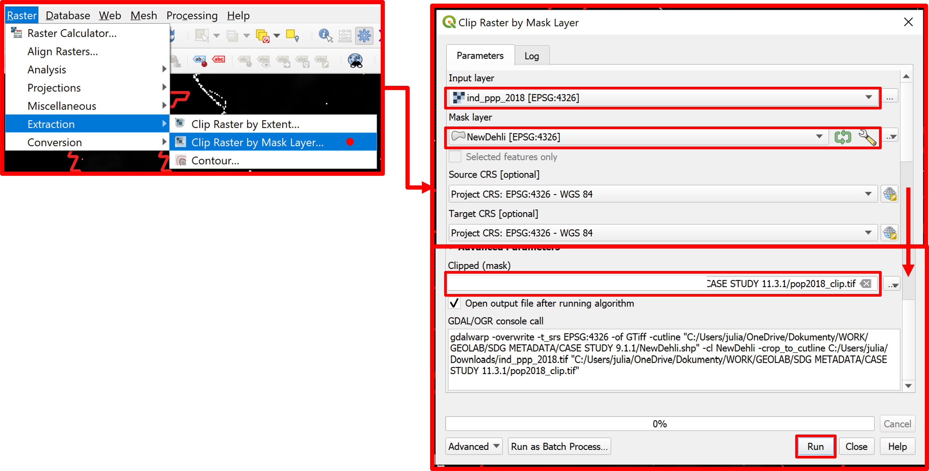
Fig. 4.2.18 Clipping the population layer for the year 2018 to New Delhi’s boundaries. Repeat the process for the 2019 layer

Use the “Zonal Statistics” tool to calculate New Delhi’s population in 2018 and 2019. Select only the “Sum” statistics, which will give us the population, as shown in Fig. 4.2.19.

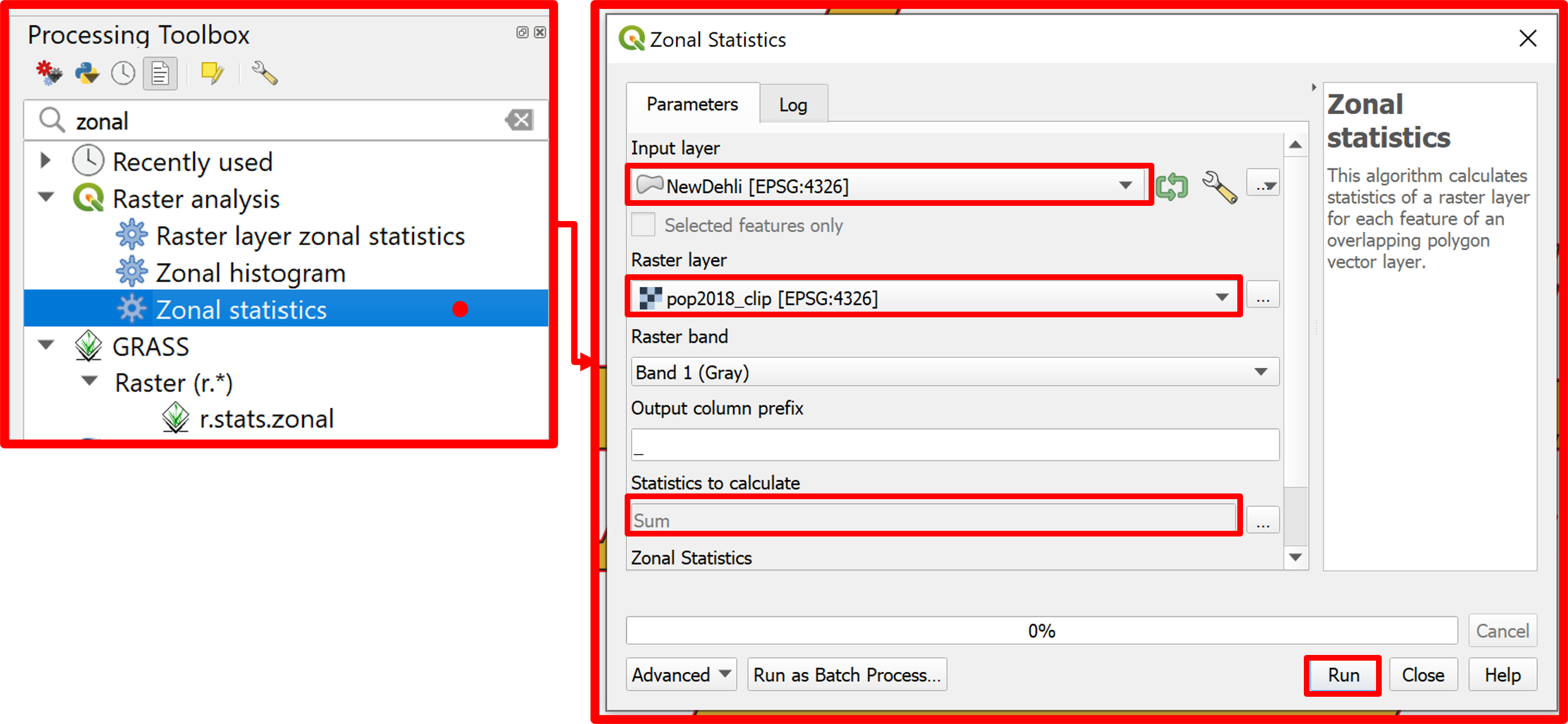
Fig. 4.2.19 Calculating New Delhi’s population in 2018. Repeat for the 2019 layer

After the previous step we’ll obtain two layers for both years. To make the computations easier we want to have the population field for both years in one layer. To do so add a new column “population_2019” to the 2018 population zonal statistics layer. Then copy the content of the “_sum” field from the 2019 population zonal statistics layer to the newly created column in the 2018 layer (Fig. 4.2.20).

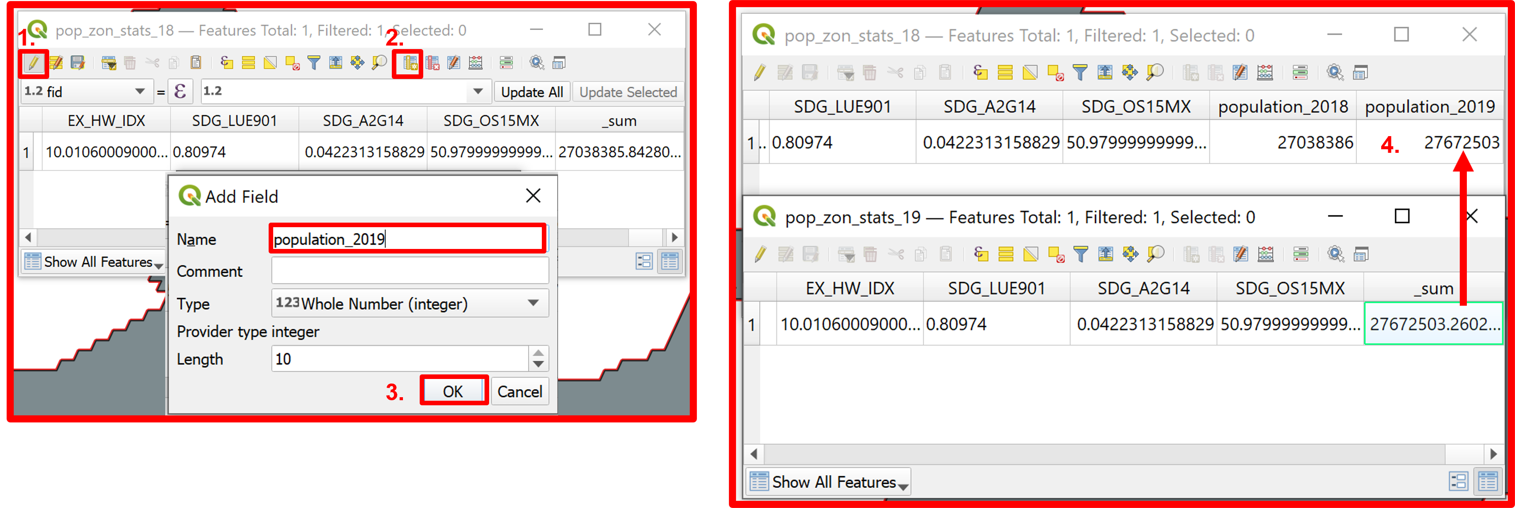
Fig. 4.2.20 Adding the population of 2019 to the 2018 zonal statistics layer

To change the name of a field in the attribute table go to the “Properties” of the layer and in the “Field” section activate the editing option (pencil icon). Now you can change the name of the “_sum” column to “population_2018” (Fig. 4.2.21).

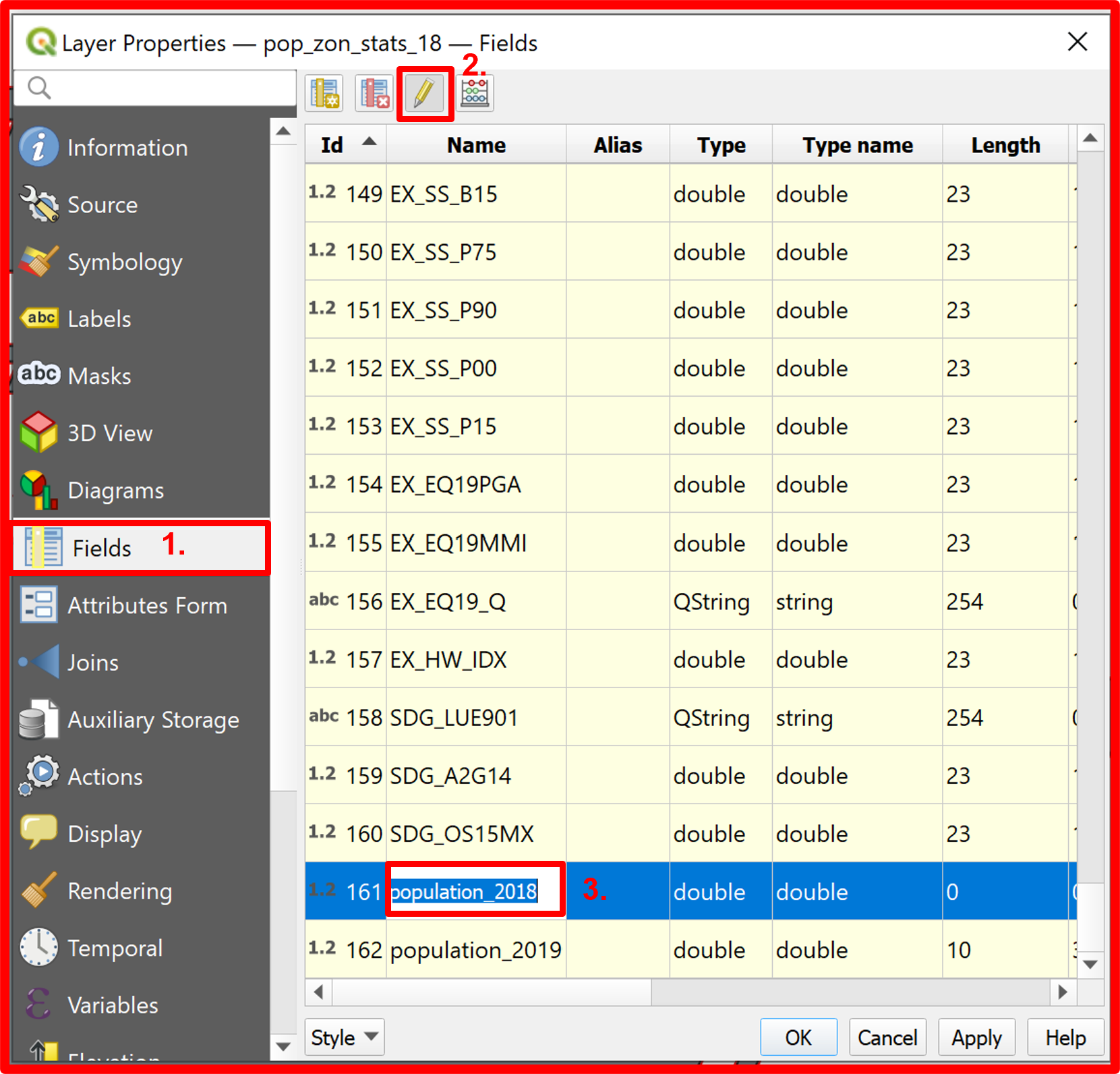
Fig. 4.2.21 Changing the name of a field in a layer’s attribute table

Now that we have the population values for both years in one layer we can calculate the PGR using the “Field Calculator” tool. Create a new field where you’ll calculate the PGR value using the before mentioned formula as shown in Fig. 4.2.22.

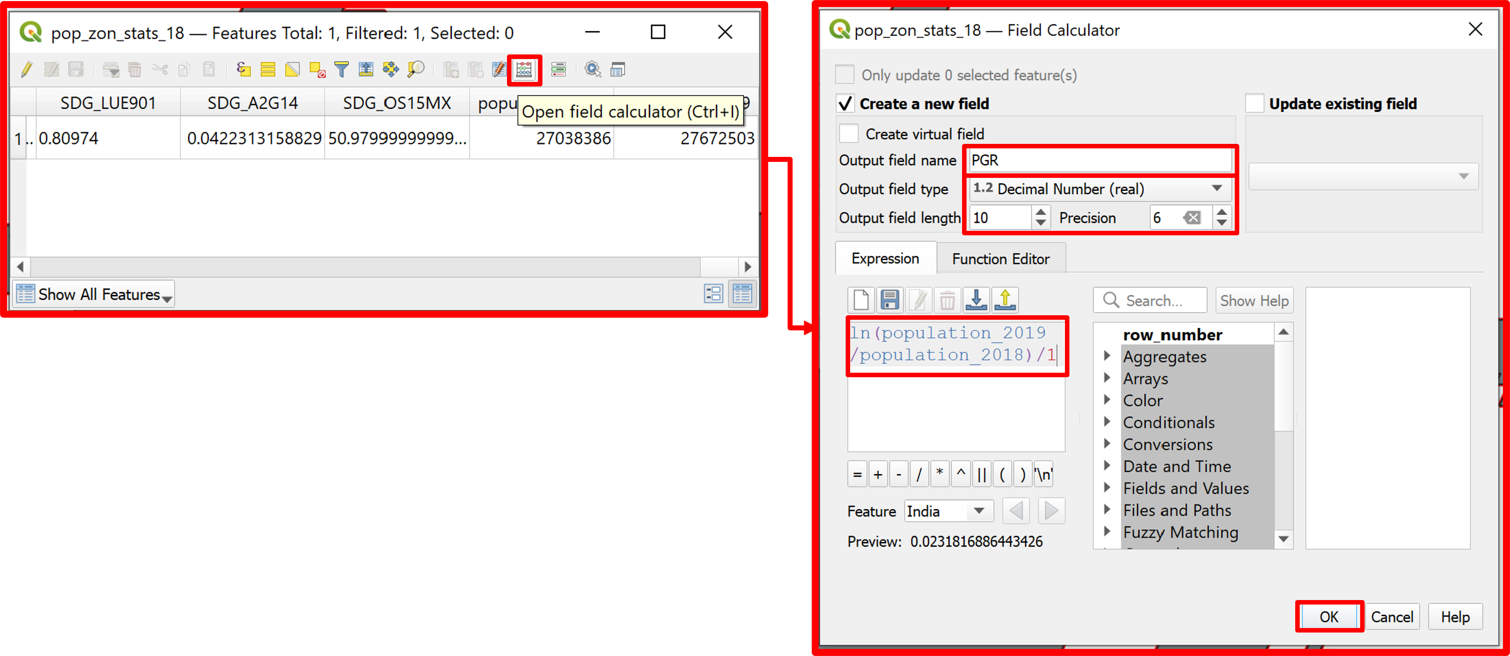
Fig. 4.2.22 Calculating the PGR index

To have both the PGR and the LCR indexes in one layer, add a new field named “PGR” in the attribute table of the “zonal_stats_2018” layer containing the previously calculated LCR (Fig. 4.2.23).

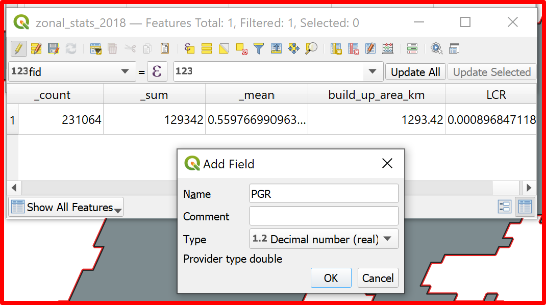
Fig. 4.2.23 Adding the PGR field into the “zonal_stats_2018” layer

5. Having the LCR and the PGR in the “zonal_stats_2018” layer we can calculate the SDG indicator 11.3.1 in the same layer by dividing the LCR by the PGR.

To calculate the indicator we will use once again the field calculator as shown in Fig. 4.2.24.

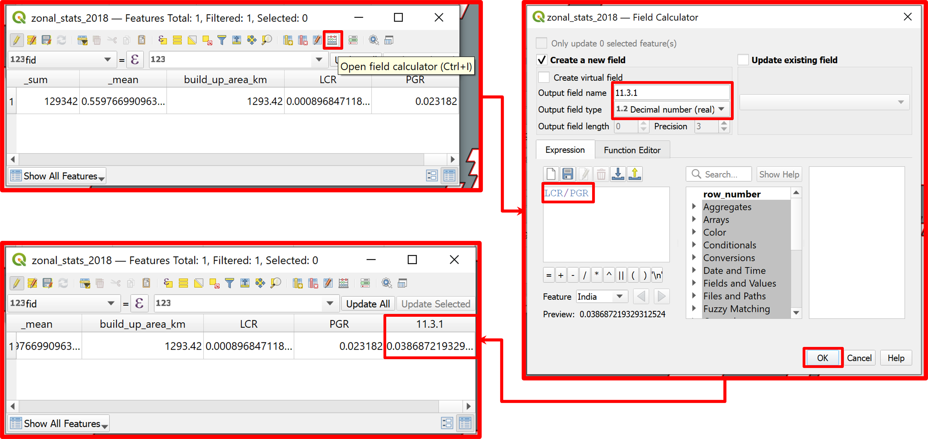
Fig. 4.2.24 Calculating the SDG indicator 11.3.1

For New Delhi the 11.3.1 indicator was estimated to be around 0.0387 in the 2018-2019 period.