4.3. Proportion of the rural population who live within 2 km of an all-season road [9.1.1]

This exercise’s purpose is to show how to compute the SDG indicator 9.1.1 defined as the share of a country’s rural population living within 2 km of an all-season road. This indicator is also commonly known as the Rural Access Index (RAI). To calculate the indicator it is needed to compute the ratio between the rural population within a 2 km buffer of an all-season road and the total rural population of the country. To compute this indicator we need three different geospatial datasets:

• The country’s population distribution, that can be retrieved from WorldPop;

  • From which it is necessary to extract only the rural population, which can be done using a Rural-Urban global definition provided by the Global Human Settlement Layer;

• The road network with road types attribute, which can be accessed for all countries from OpenStreetMap;

For more information about the background of the SDG indicator 9.1.1 refer to the metadata provided here link.

In this exercise we will calculate the indicator for Gabon in 2020.

First, we need to download all the necessary data:

• From https://hub.worldpop.org/geodata/listing?id=78 download the population raster layer for Gabon in 2020 as shown in Fig. 4.3.1.

  • From https://ghsl.jrc.ec.europa.eu/ghs_stat_ucdb2015mt_r2019a.php download the Urban Centre Database (Fig. 4.3.2)

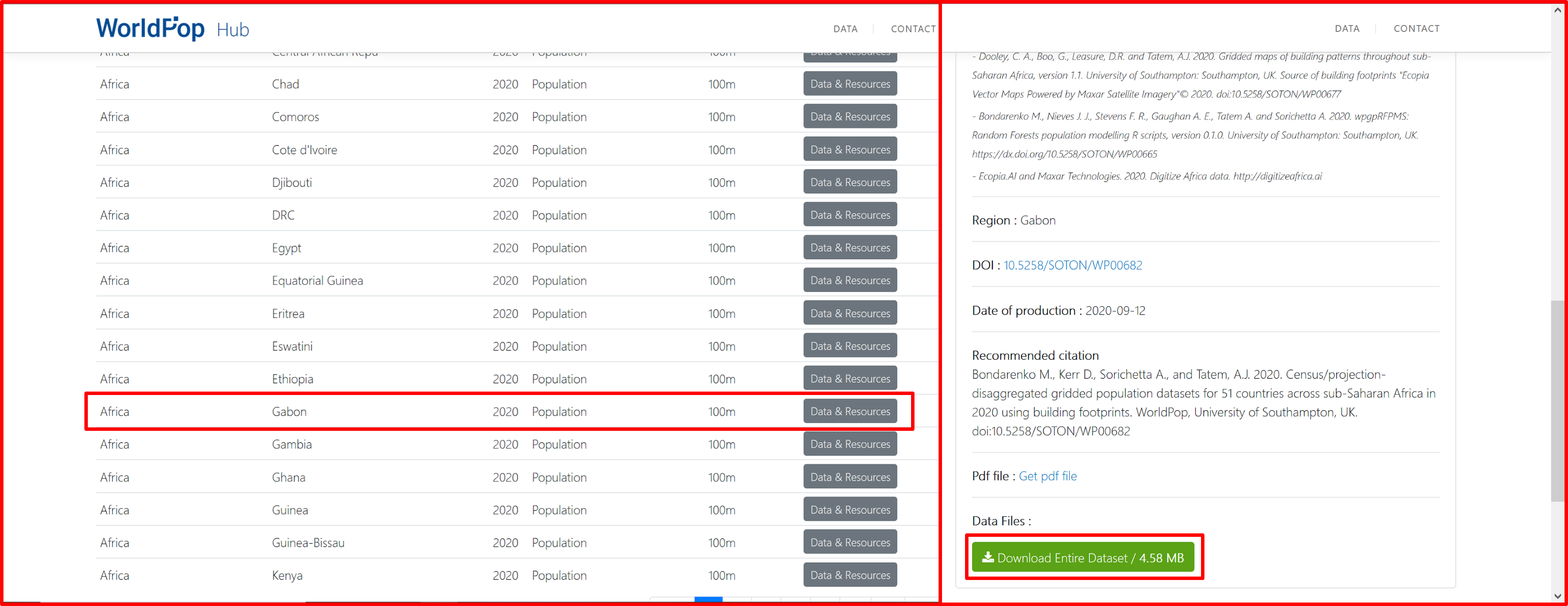
Fig. 4.3.1 Downloading the population raster layer of Gabon 2020

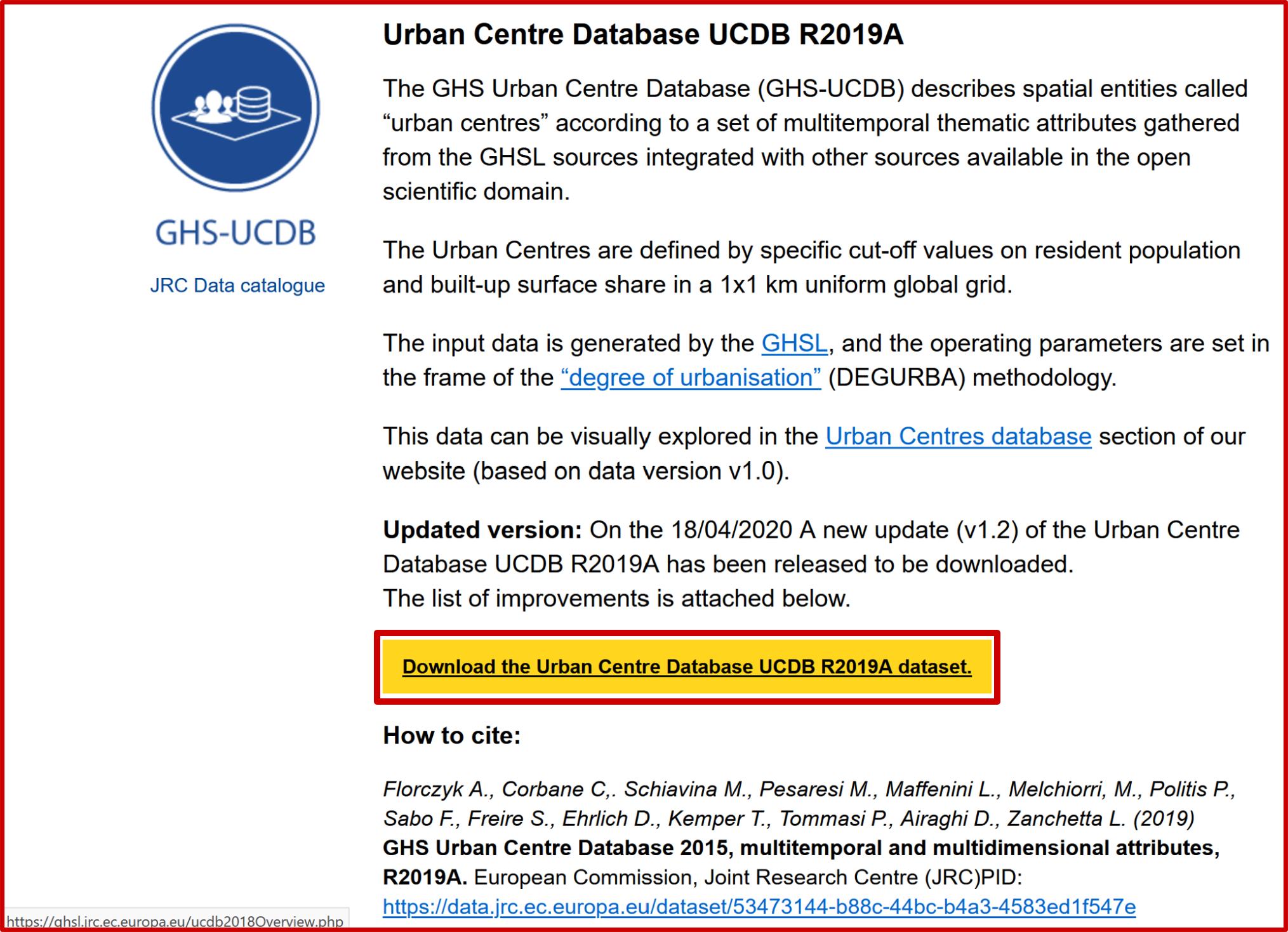
Fig. 4.3.2 Downloading the delimitation of urban areas file

• From https://download.geofabrik.de/africa/gabon.html download the OSM data. After that unpack the .zip file and keep only the files related to the road network (”gis_osm_roads_free”). The procedure is shown in Fig. 4.3.3

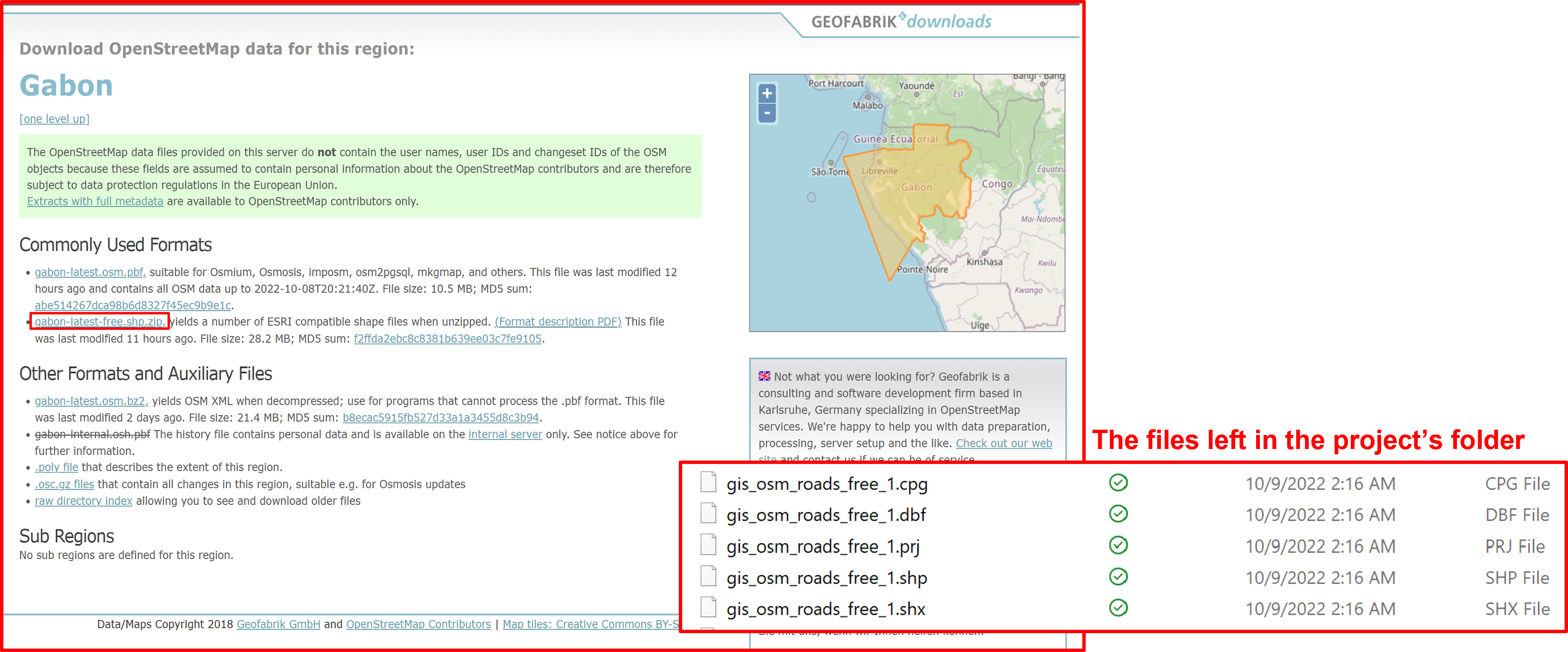
Fig. 4.3.3 Downloading the road network data from OSM.

Open a new QGIS project and add the road network shapefile (Fig. 4.3.4) and the downloaded population grid file (Fig. 4.3.5).

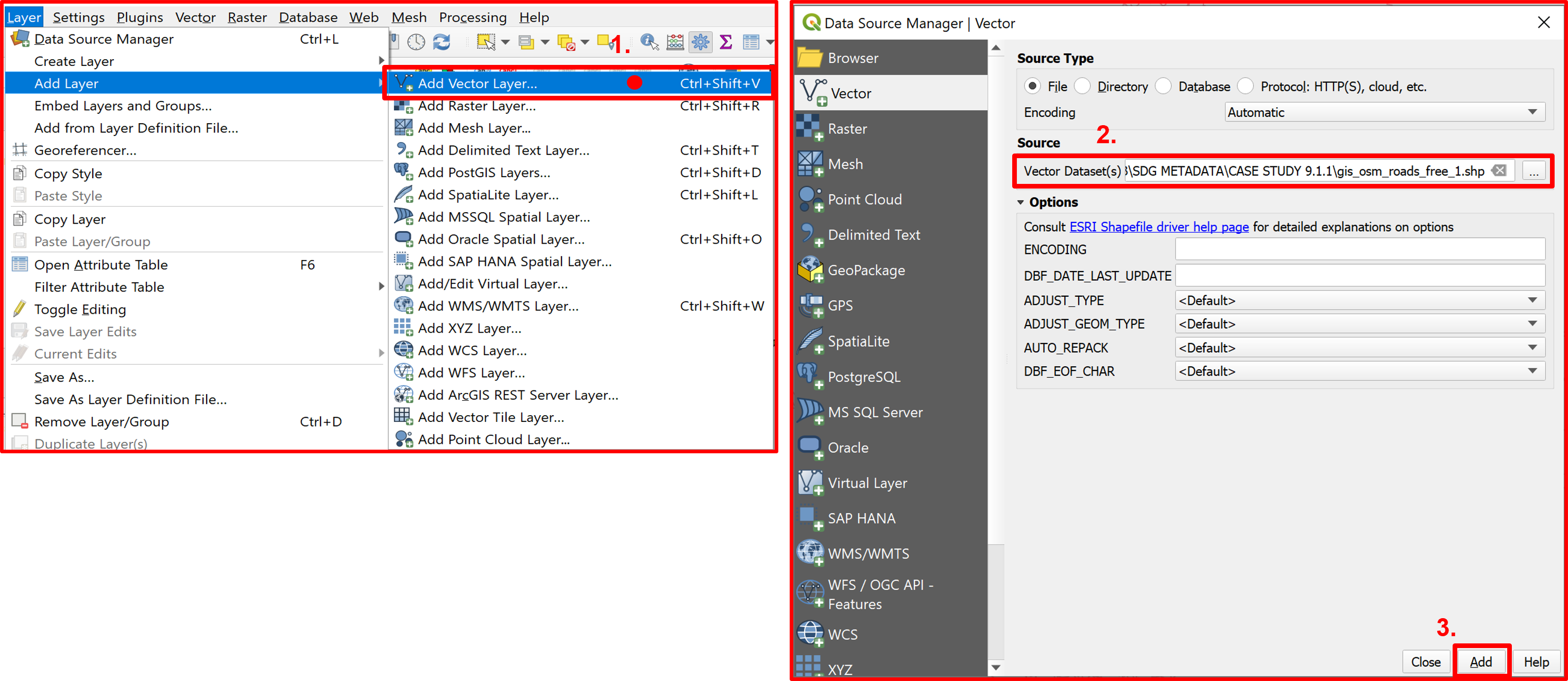
Fig. 4.3.4 Adding the vector layer of the Gabon road network to the QGIS project

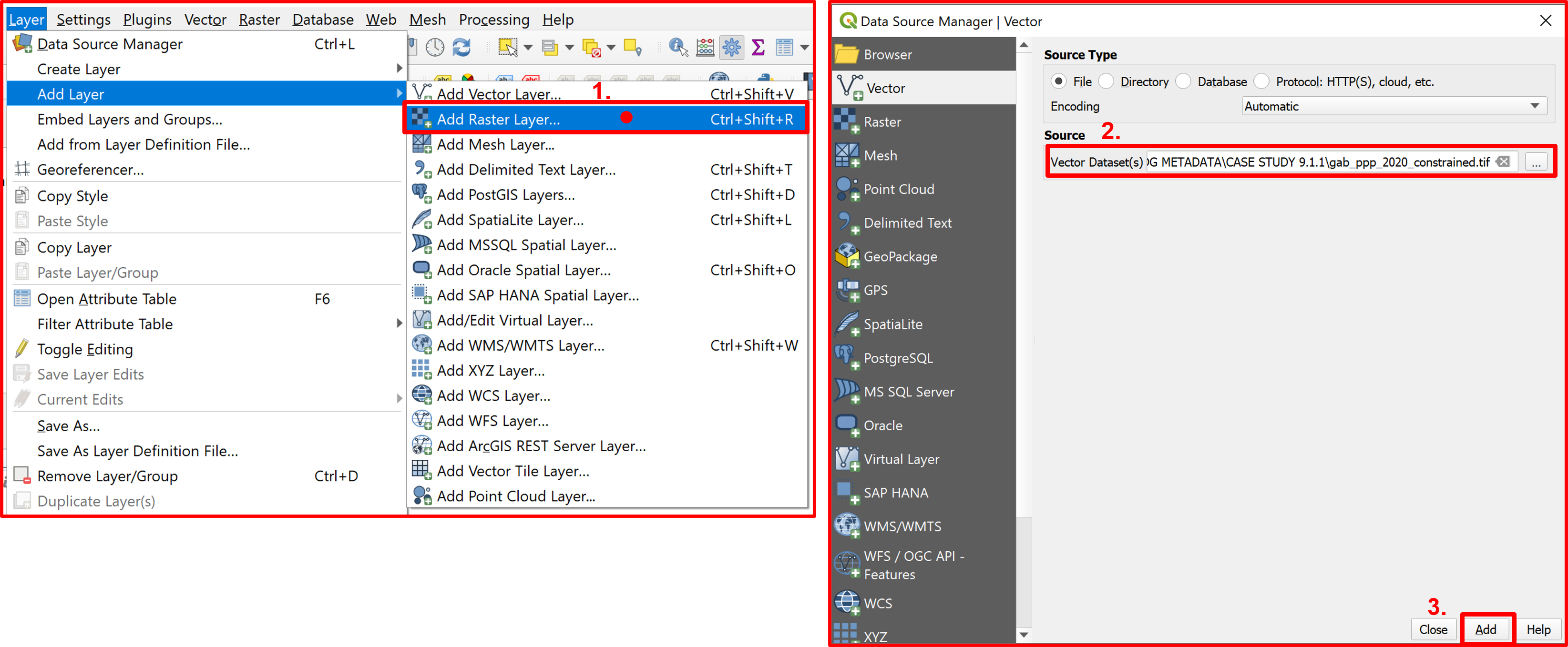
Fig. 4.3.5 Adding the Gabon population raster layer to the QGIS project

Since we are interested only in all-season, major roads we need to extract only those from the shapefile vector layer. The information about the codes for the roads from the “Format Specification” for OSM data (Fig. 4.3.6) indicates that the major roads have codes starting with 511.

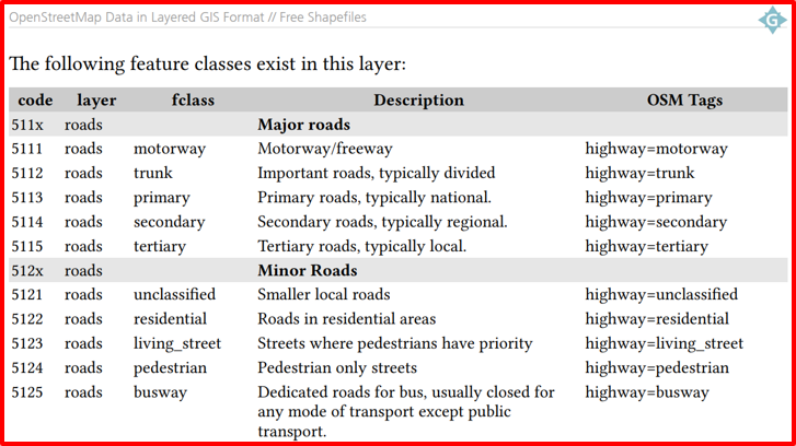
Fig. 4.3.6 “Format Specification” regarding OSM roads’ codes

Using the selection by expression, we can select the roads with codes that are smaller than 5120 as shown in Fig. 4.3.7. After the selection of major roads we want to export them in a new vector layer that will be called “all_season_roads.shp”.

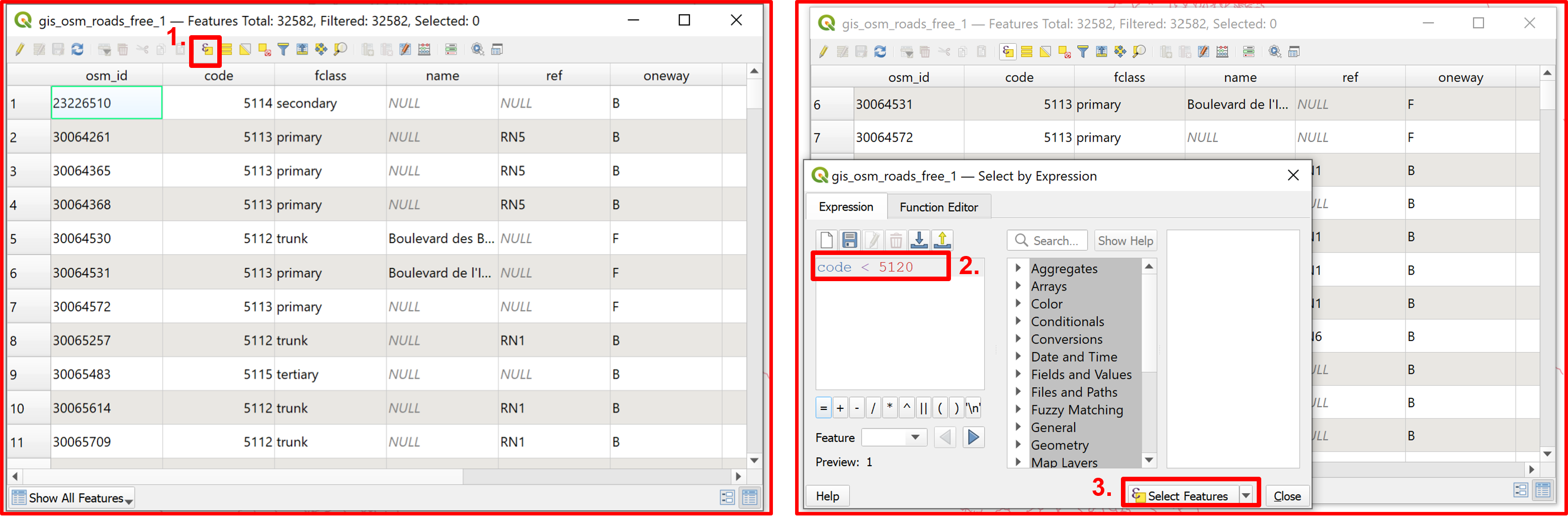
Fig. 4.3.7 Selecting major roads in Gabon

The procedure of extracting selected features is presented in Fig. 4.3.8, and the expected view after the procedure is shown in Fig. 4.3.9.

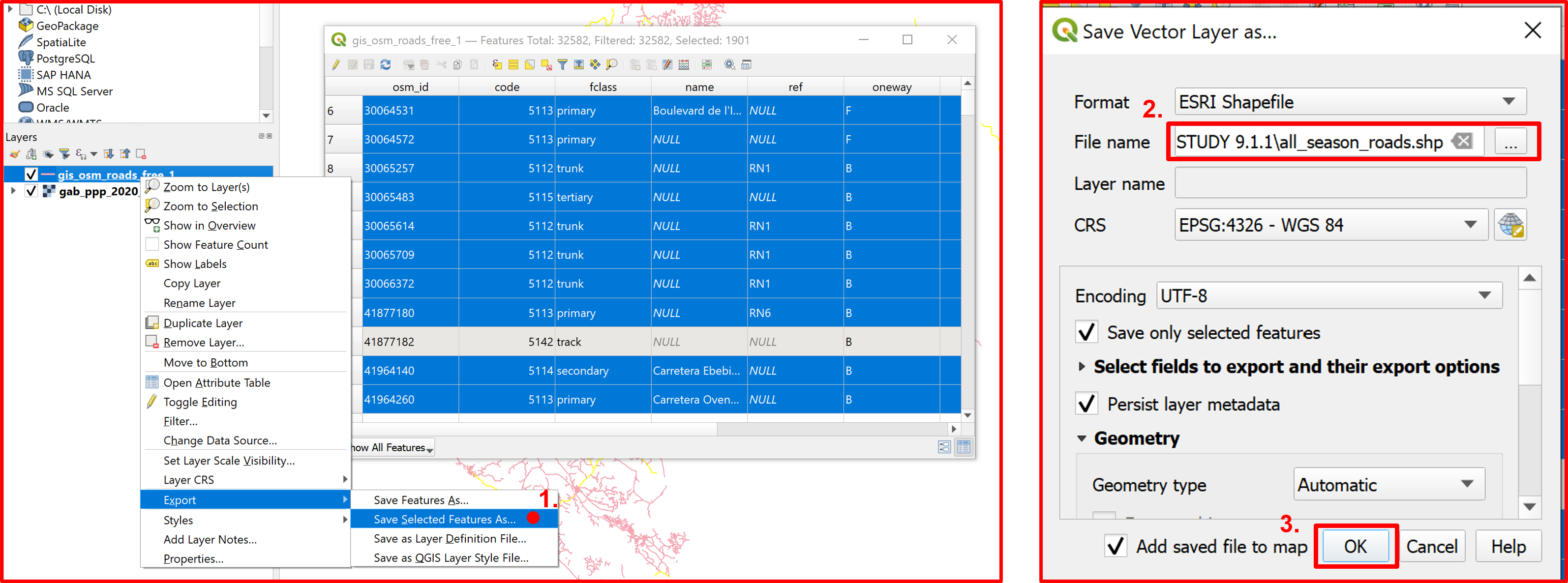
Fig. 4.3.8 Extracting the selected features

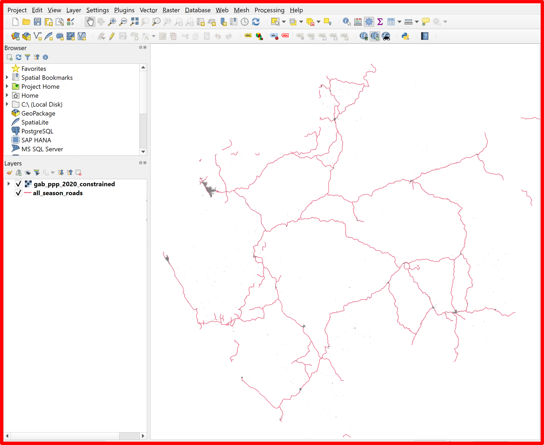
Fig. 4.3.9 Expected view after extracting only Gabon’s major roads.

We now need to create the 2 km buffer around the major roads, by using the “Buffer” geoprocessing tool (Fig. 4.3.10). Because of reprojecting issues that may be encountered we input the distance in degrees.

Warning

To work with metric buffer distance units, reproject all the layers in the correct UTM zone.

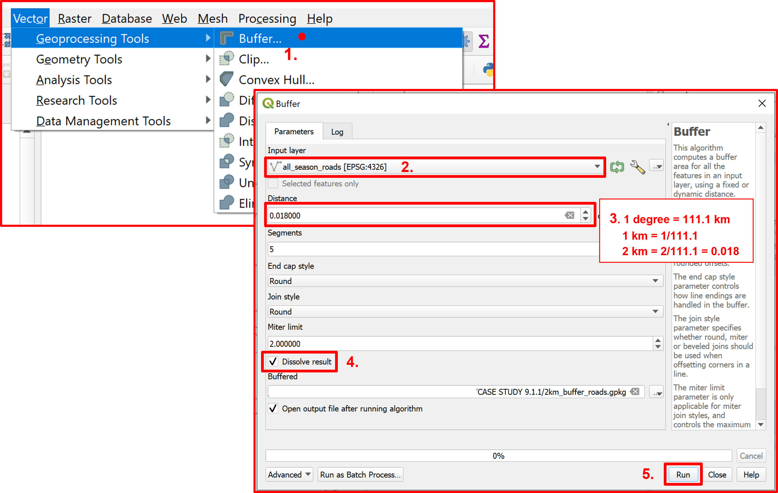
Fig. 4.3.10 Creating a 2 km buffer around the major roads

Now we have the buffer around the major roads and the population grid of Gabon. We want to extract just the rural population within that buffer, hence we need to exclude the urban areas from the computations. To do so add the urban extent layer previously downloaded (Fig. 4.3.11) and compute the difference between the previously created road buffer and the urban extent layer (Fig. 4.3.12). This will create a new vector layer containing the buffer only in rural areas.

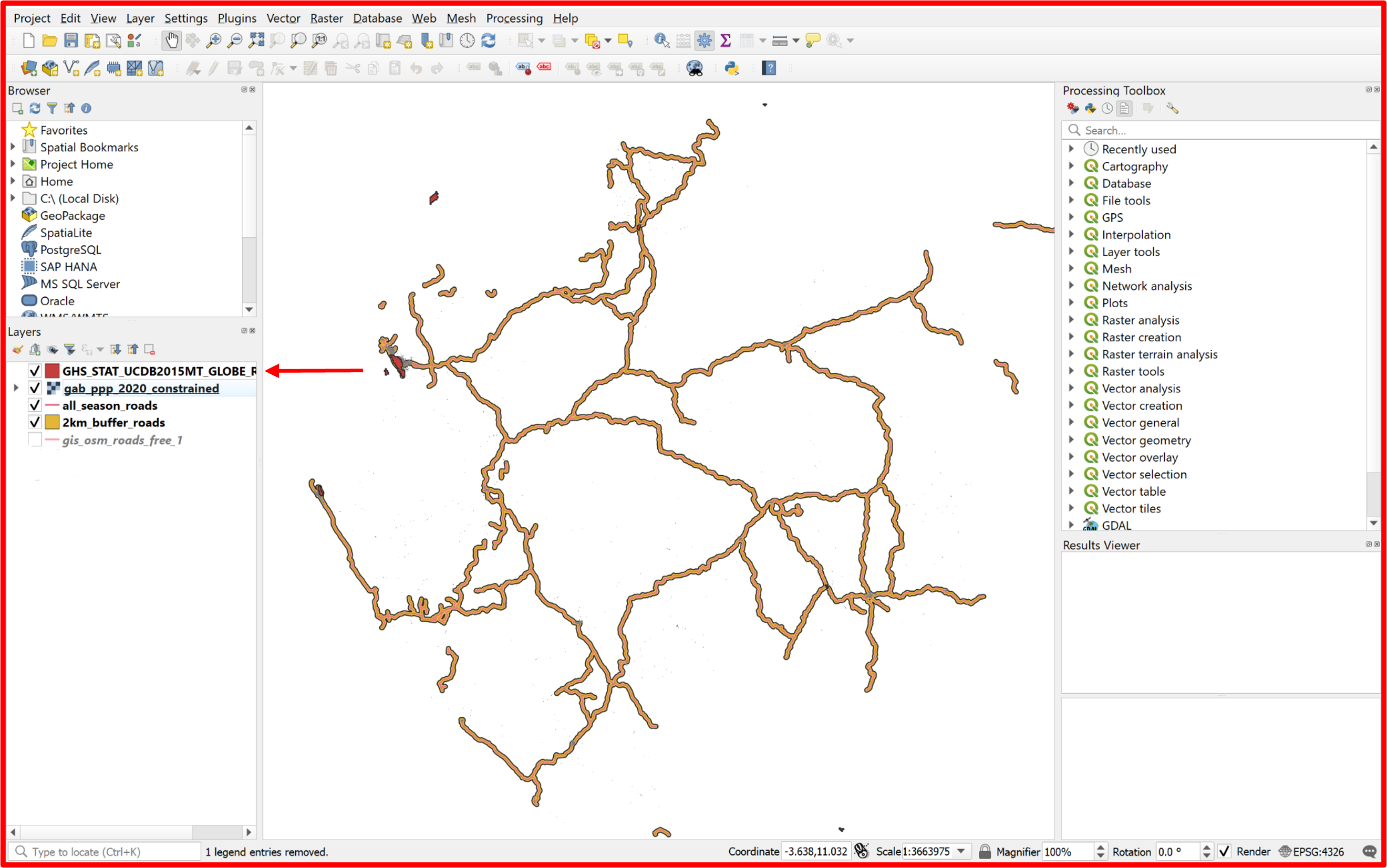
Fig. 4.3.11 Adding the urban extent vector layer to the QGIS project

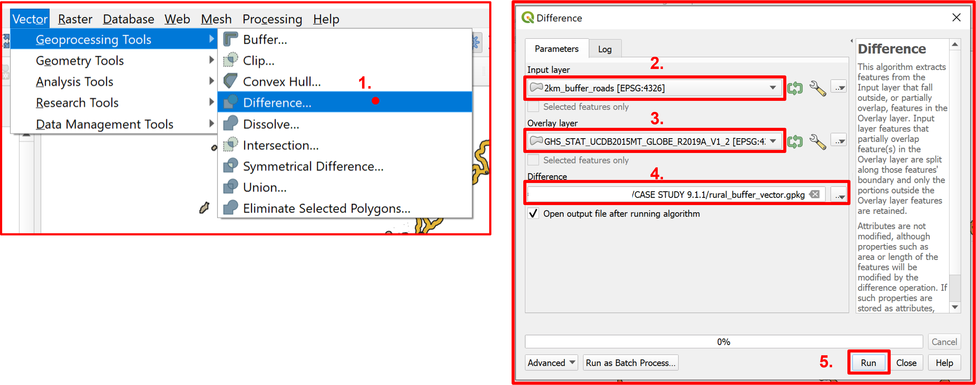
Fig. 4.3.12 Subtracting the urban extent layer from the road buffer layer

Warning

In case of “Invalid Geometry” error: click the wrench icon by the side of the overlay layer and select “Do not Filter (Better Performance)” from the drop down menu in the “Invalid feature filtering” option.

Having this vector layer and the population grid layer we will use them as input layers to calculate the rural population within the 2 km buffer of a major road by using the “Zonal Statistics” tool (Fig. 4.3.13).

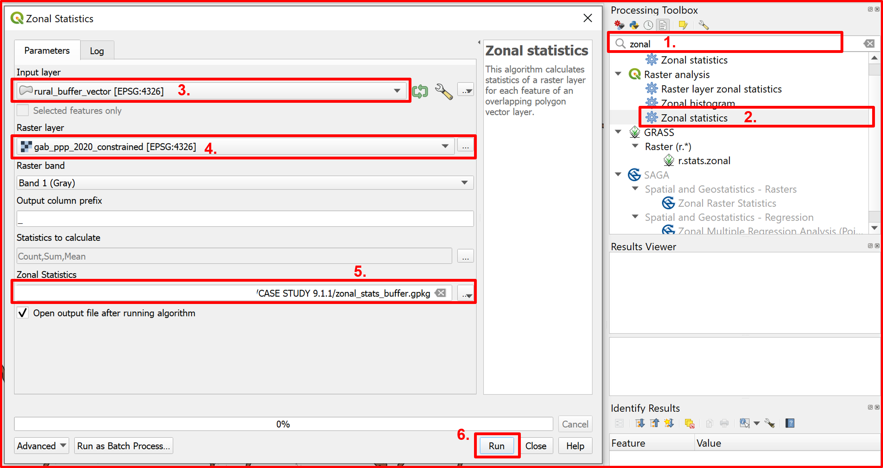
Fig. 4.3.13 Calculating the rural population within the 2 km buffer around major roads.

After this step we have the rural population within a 2 km buffer of a major road (Fig. 4.3.14).

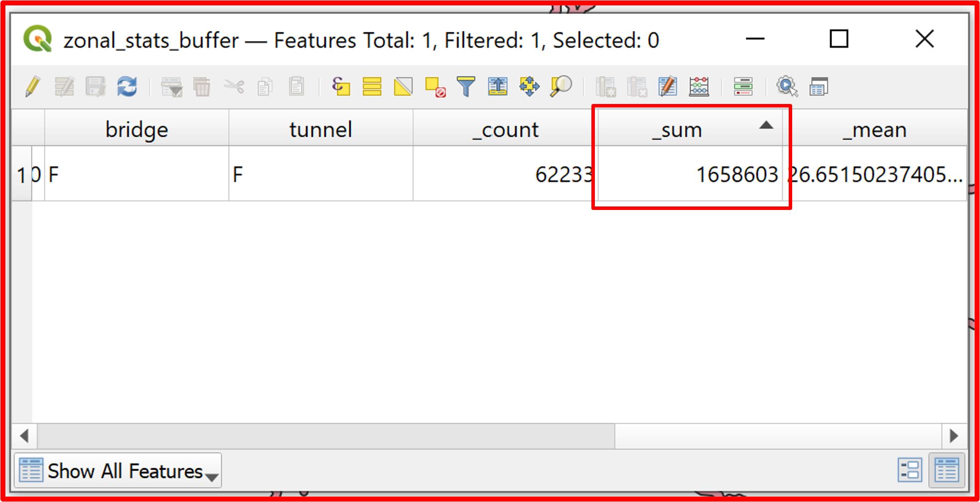
Fig. 4.3.14 Restult of the “zonal statistics” operation

To calculate the indicator 9.1.1 we also need the total rural population of Gabon, which we will calculate in the next steps. Firstly, we need Gabon’s boundaries to delimitate the urban extent layer ust to our area of interest. To retrieve this data go to https://datacatalog.worldbank.org/search/dataset/0038272 and download the “World Country Polygons - Very High Definition” as shown in Fig. 4.3.15.

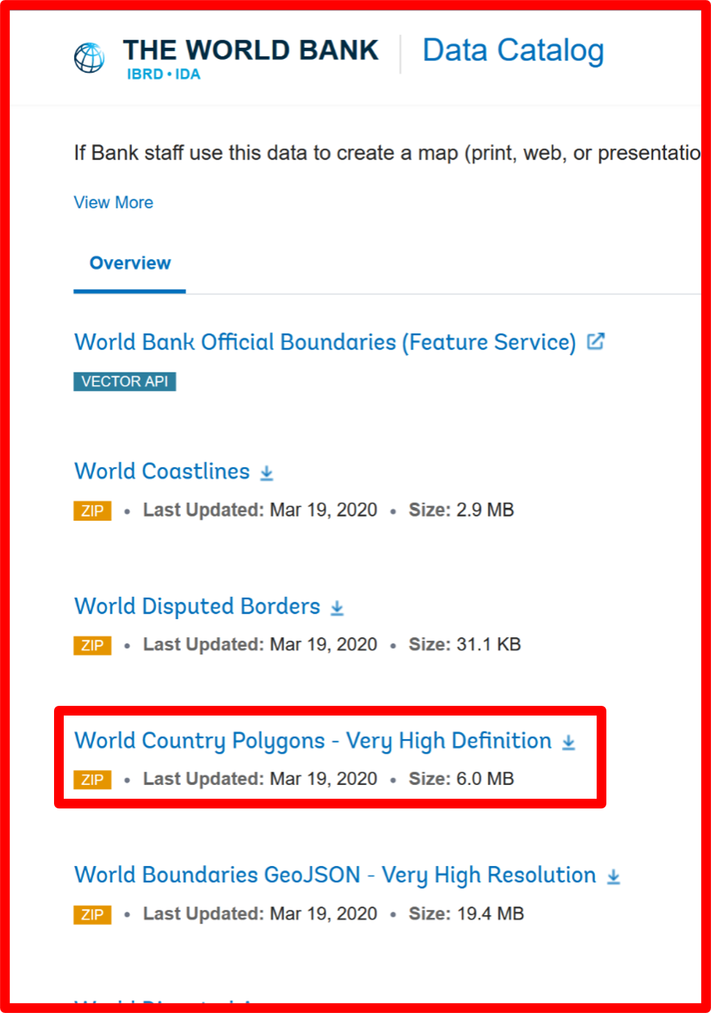
Fig. 4.3.15 Downloading the “World Country Polygons”

Add the downloaded shapefile to the QGIS project (Fig. 4.3.16).

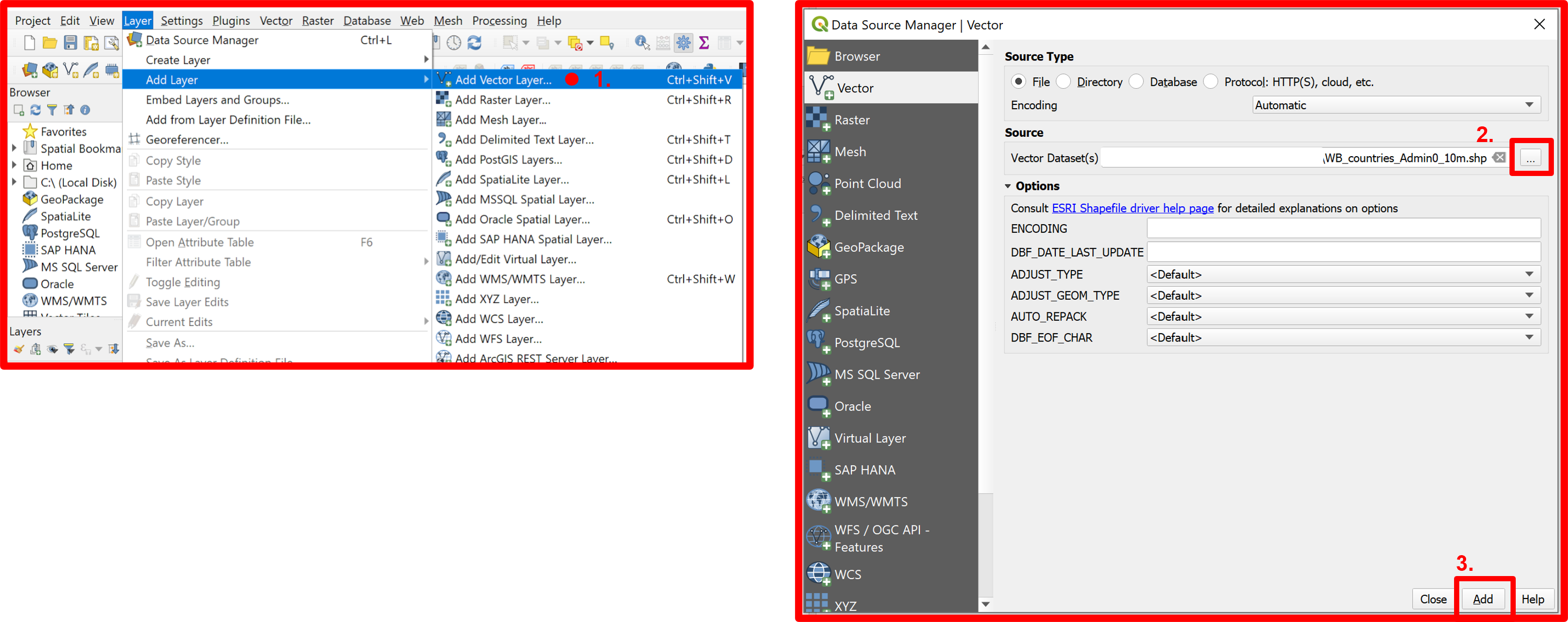
Fig. 4.3.16 Adding the countries’ boundaries vector layer to the QGIS project

Since we are interested only in the boundaries of Gabon we need to extract them from the vector file. To do so select Gabon’s polygon by area as presented in Fig. 4.3.17.

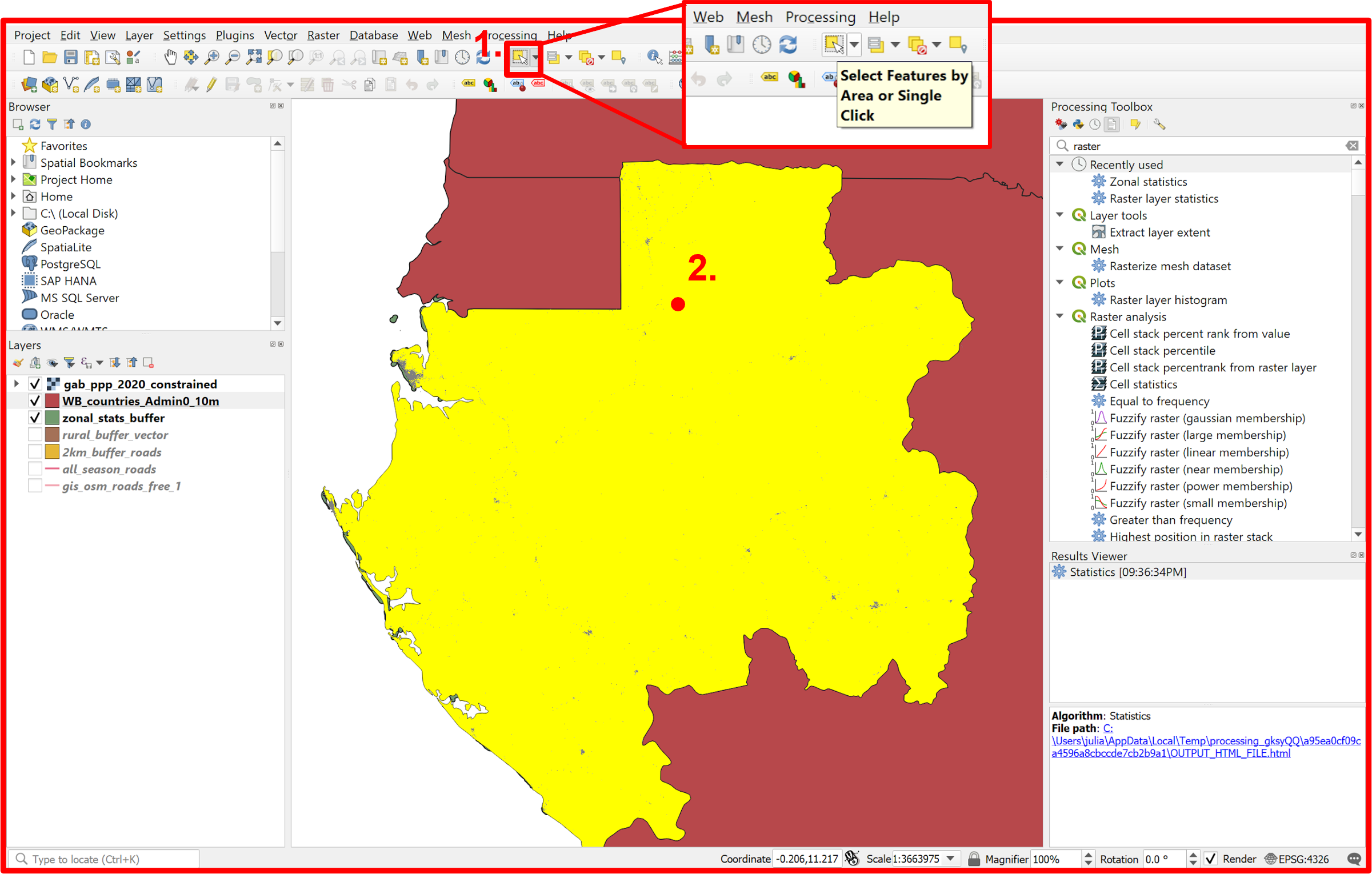
Fig. 4.3.17 Selecting Gabon by area

Now extract the selected feature to a new vector layer “Gabon.shp” (Fig. 4.3.18).

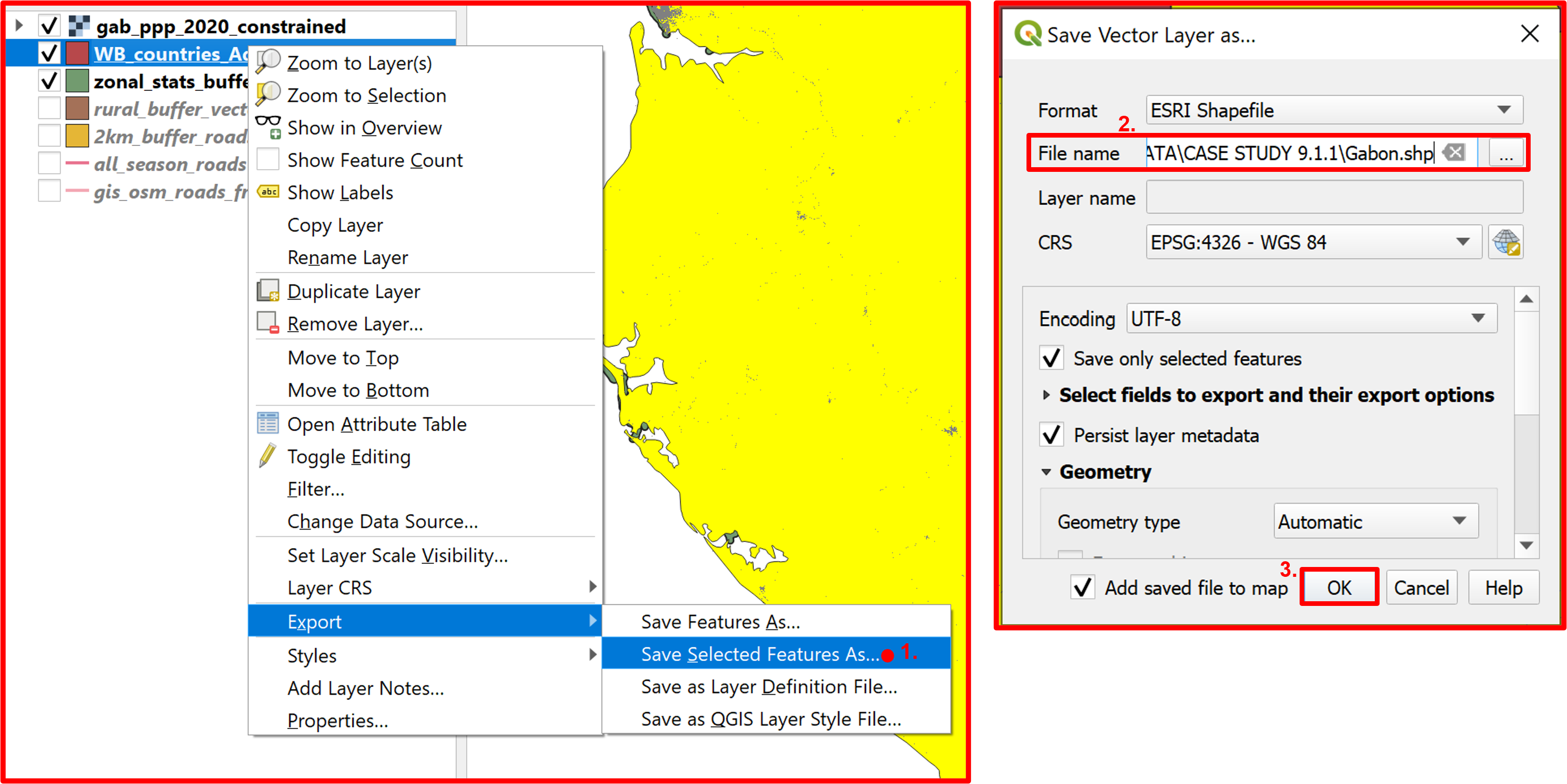
Fig. 4.3.18 Extracting the selected Gabon polygon

For better visualization purposes change the symbology of the new layer in its “Properties”, which can be accessed by right clicking the layer in the layers panel. An example of a clear symbology for a country’s boundaries is presented in Fig. 4.3.19.

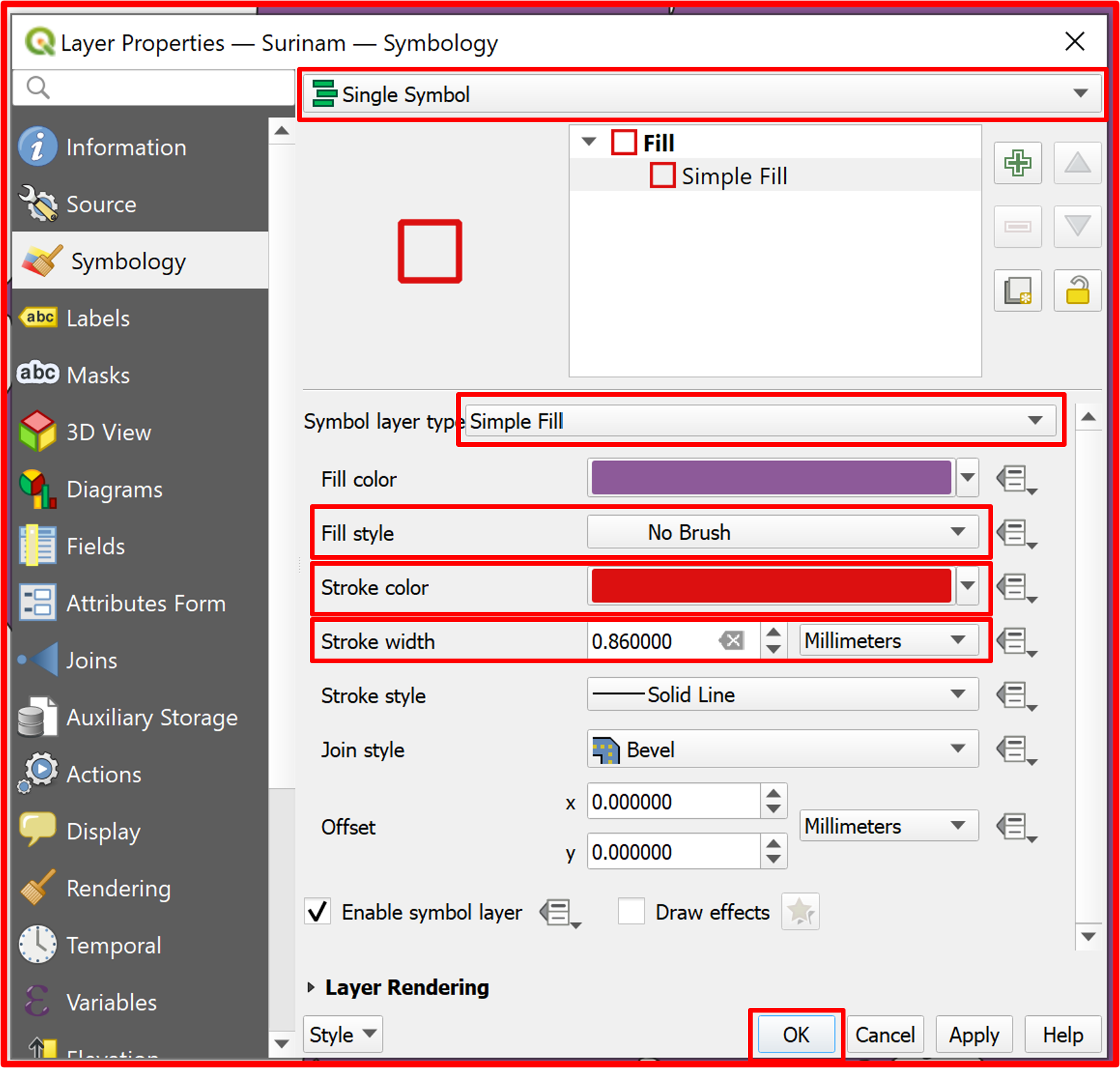
Fig. 4.3.19 Changing the “Gabon.shp” symbology

Now we can clip the urban extent layer to Gabon’s borders by using the “Clip” geoprocessing tool (Fig. 4.3.20).

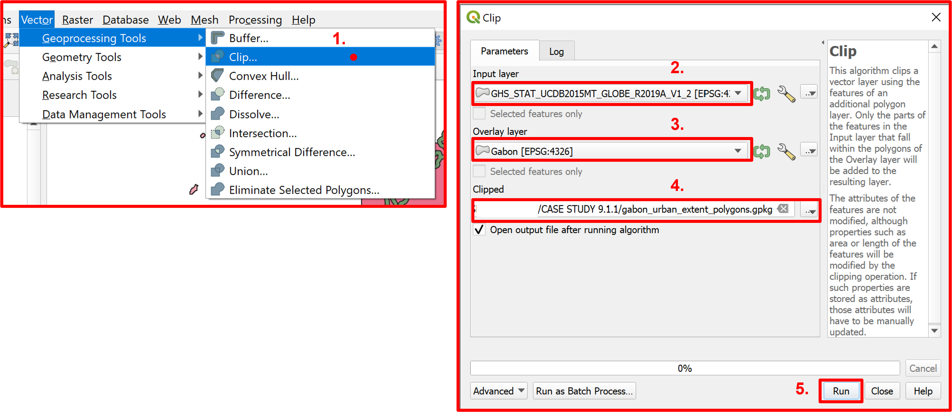
Fig. 4.3.20 Clipping the urban extent layer to Gabon’s extent

The urban extent polygons are now limited only to Gabon’s extent. If we open the attribute table now, we can see that for each urban area there’s a distinct row. Since we are interested in the urban areas as a whole we want to have just one record for all the urban areas in Gabon. To do so we need to use the “Dissolve” geoprocessing tool as shown in Fig. 4.3.21.

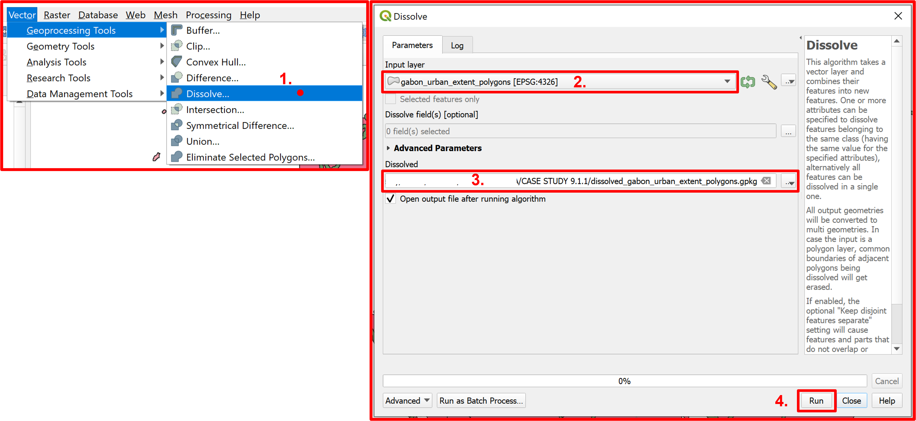
Fig. 4.3.21 Dissolving the urban extent layer

The attribute table of the Gabon’s urban extent layer after this operation can be found in Fig. 4.3.22.

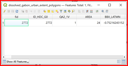
Fig. 4.3.22 The expected result of the “Dissolve” procedure

We can now easily calculate the total urban population with “Zonal Statistics”, in the newly created vector layer the “_sum” field presents the total urban population of Gabon (Fig. 4.3.23).

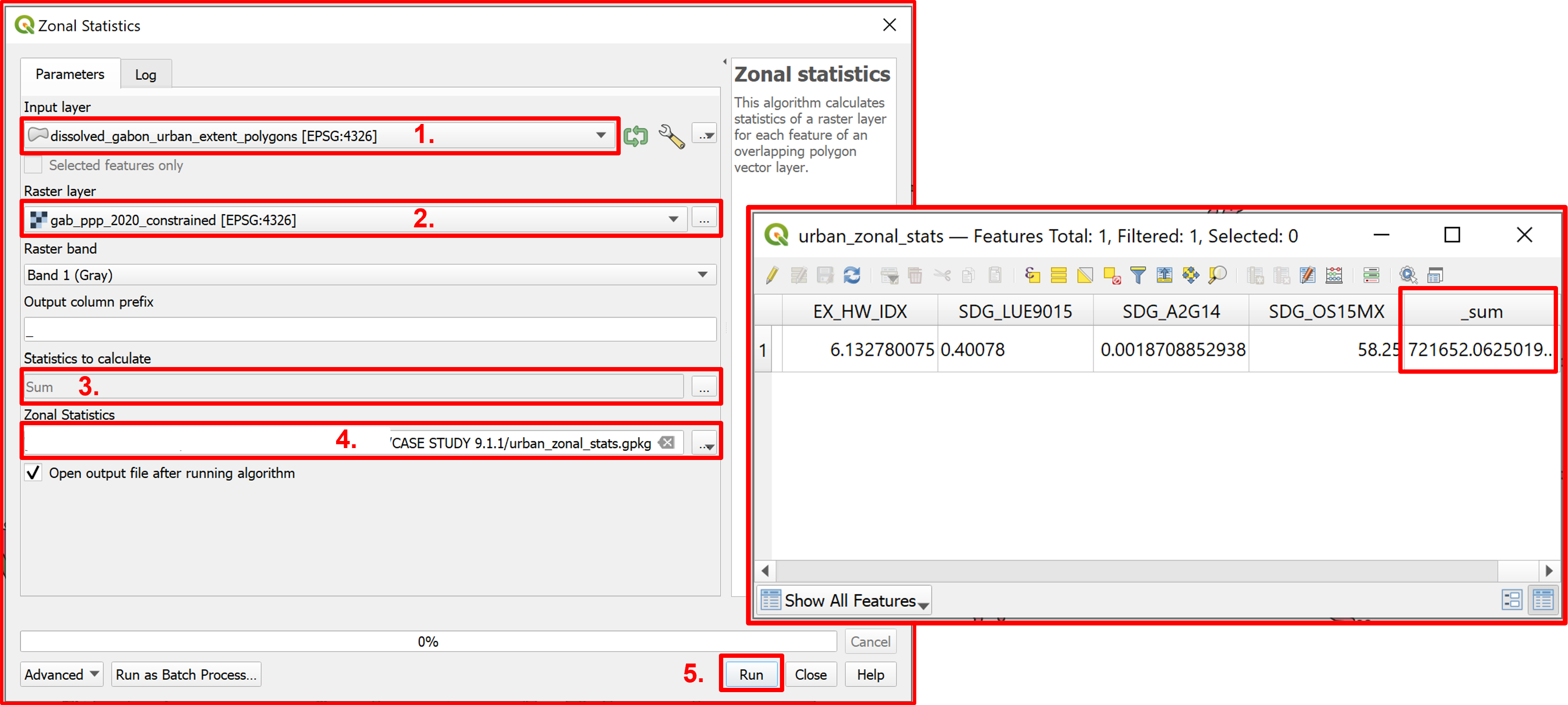
Fig. 4.3.23 Calculating the total urban population of Gabon

To calculate the needed rural population of Gabon it is needed to first retrieve the total population, so then we can compute:

\(\text{Rural population} = \text{Total Population} - \text{Urban Population}\);

To calculate from the population grid the total population we will use the “Raster layer statistics” with the population raster layer as input. The output of this process is stored in a temporary .html file which you can find in the right bottom corner of your screen in the “Result Viewer” panel (Fig. 4.3.24).

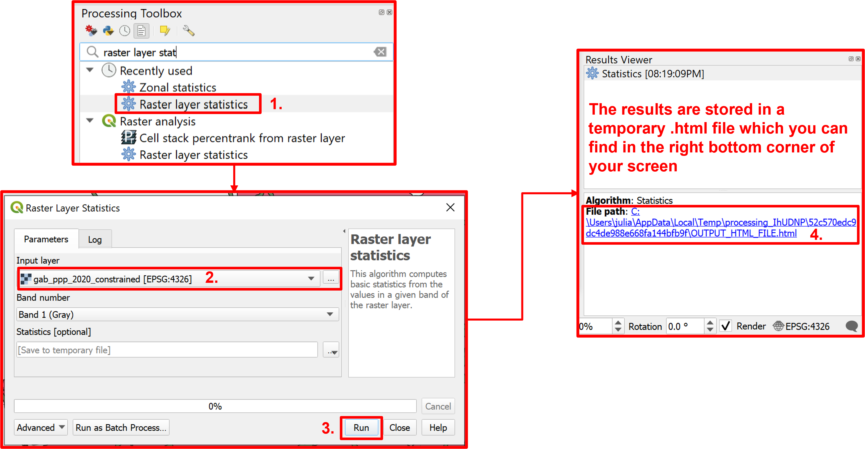
Fig. 4.3.24 Calculating the total population of Gabon in 2020 with the “Raster layer statistics”

We now have all the necessary data to calculate the indicator. To make the computations easier and faster we first need to add all the needed values into one layer. Open the attribute table of the “zonal_stats_buffer.shp” layer, which we previously created to calculate the rural population within the 2 km buffer. Start editing and add two new integer fields, one for the total population and the second for the urban population (Fig. 4.3.25).

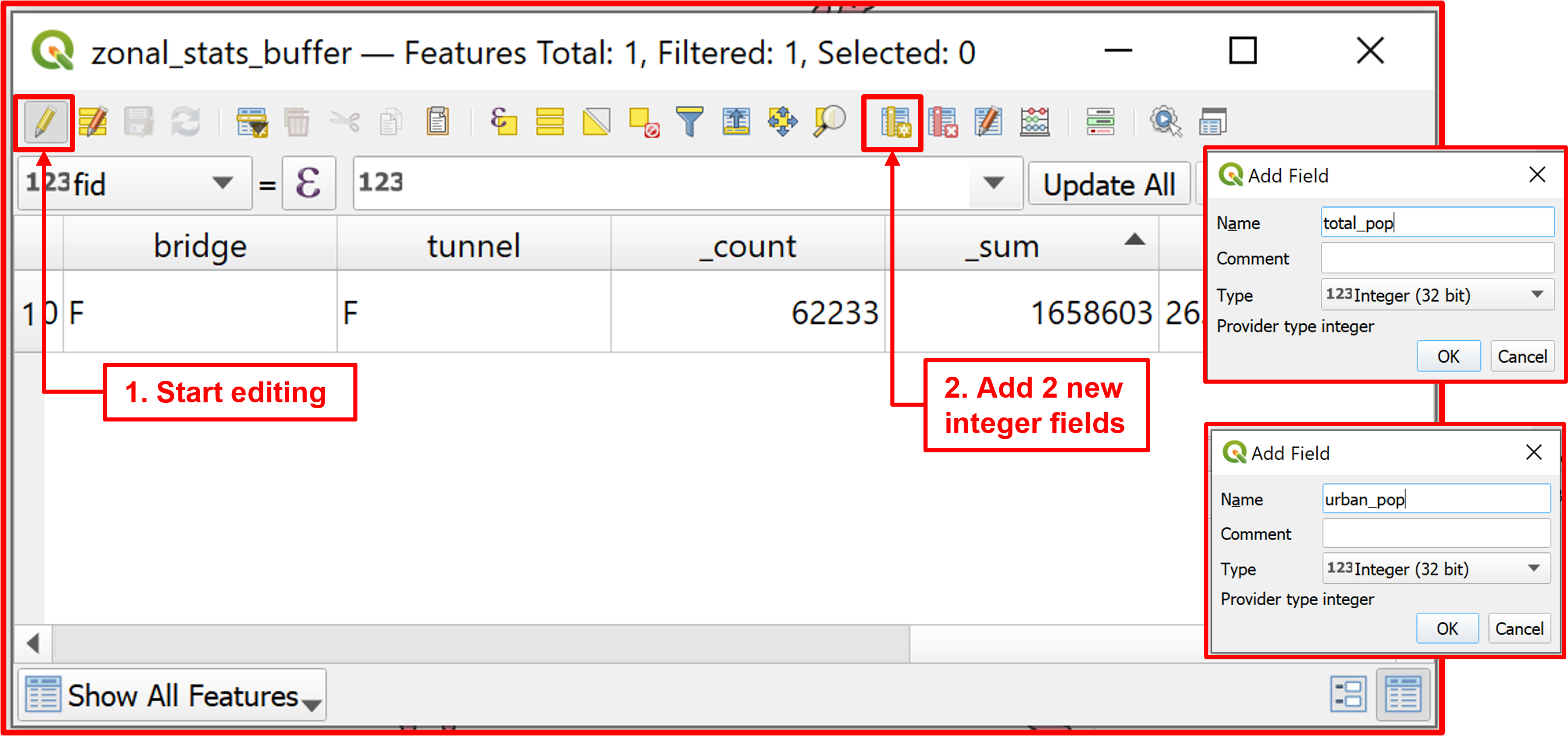
Fig. 4.3.25 Adding new fields to the attribute table of “zonal_stats_buffer.shp”

To the “total_pop” field paste the value of the “Sum” from the .html file generated by the “Raster layer statistics” tool (Fig. 4.3.26).

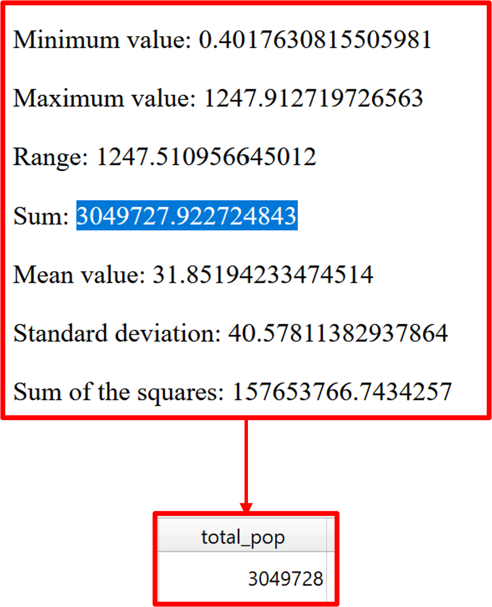
Fig. 4.3.26 Populating the “total_pop” field

To the “urban_pop” paste the value of the “_sum” field from the attribute table of the “urban_zonal_stats.shp” layer (Fig. 4.3.27).

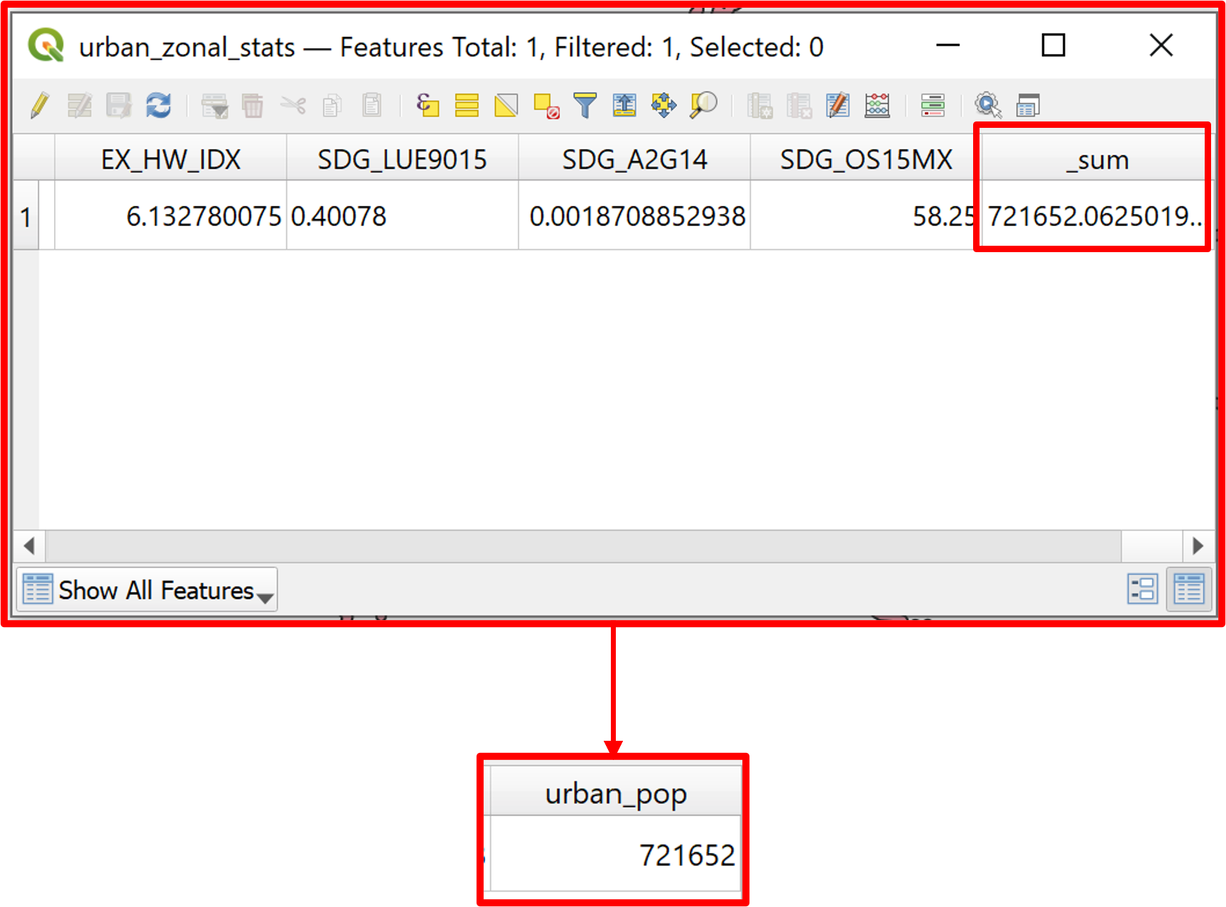
Fig. 4.3.27 Populating the “urban_pop” field

Finally, we can calculate the SDG 9.1.1 indicator using the “Field Calculator”. Since the indicator is defined as:

\(\frac{\text{Rural population living in a 2 km buffer from a major road}}{\text{Total rural population}}\)

we can compute it as shown in Fig. 4.3.28.

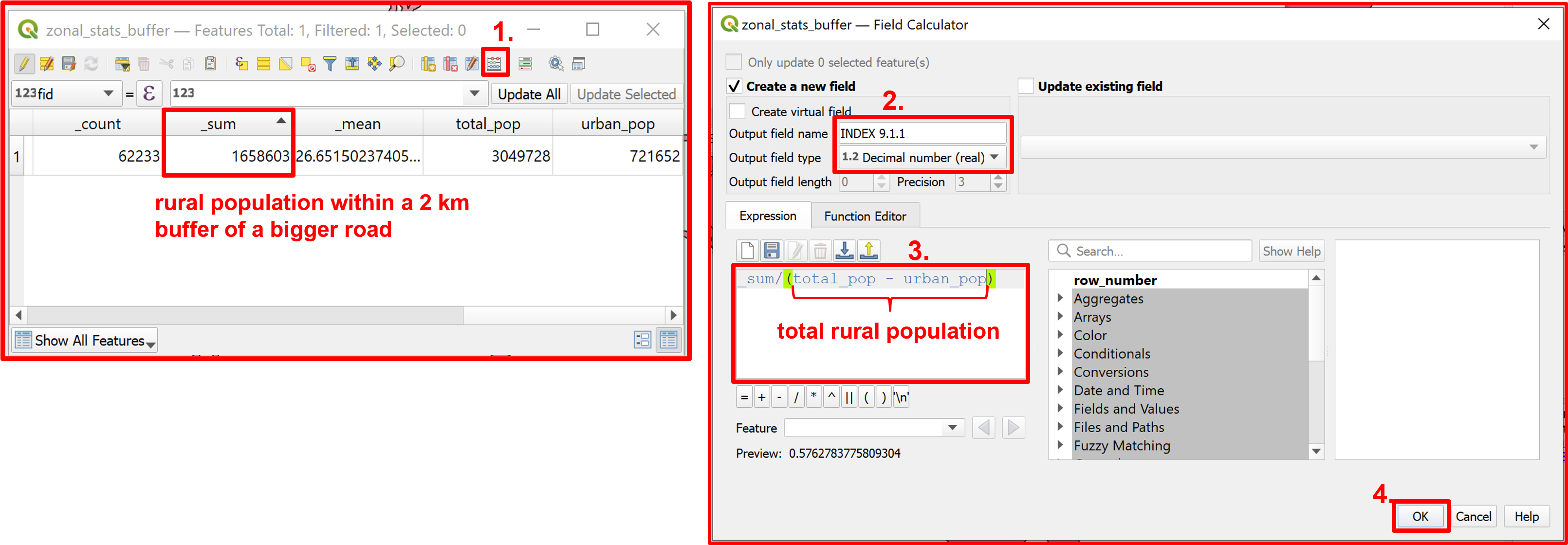
Fig. 4.3.28 Calculating of the SDG 9.1.1 indicator

The final result (Fig. 4.3.29) indicated that around 71% of Gabon’s total rural population lives in a 2 km buffer from a major, all-season road.

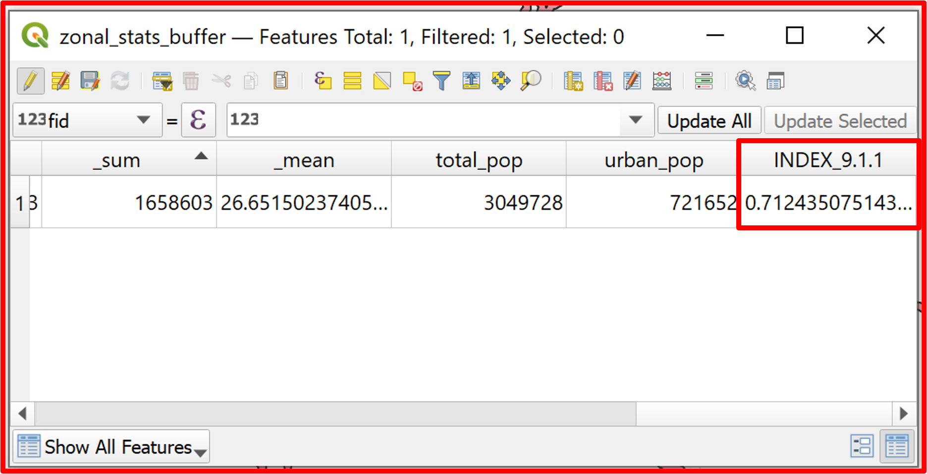
Fig. 4.3.29 The attribute table with the final result