4.1. Forest area as a proportion of total land area [15.1.1]

In this exercise you will learn how to calculate the indicator 15.1.1 which is defined as the forest area as a proportion of total land area, and is expressed in percentages. To learn more about this indicator read the metadata provided under this link. The method of computation is given by the following formula:

\(\frac{\text{Forest area (reference year)}}{\text{Land area (reference year)}} * 100\),

thus we need to first define the region and reference year for which the indicator needs to be calculated. After that, we need to estimate the forest area and land area of the region. In this case study we’ll be working on calculating the indicator for Suriname for the reference year 2019.

The first step is to download the vector data of the countries in shapefile format from the WorldBank (Fig. 4.1.1). The file contains polygons of all the world’s countries, and it will come useful in next exercises.

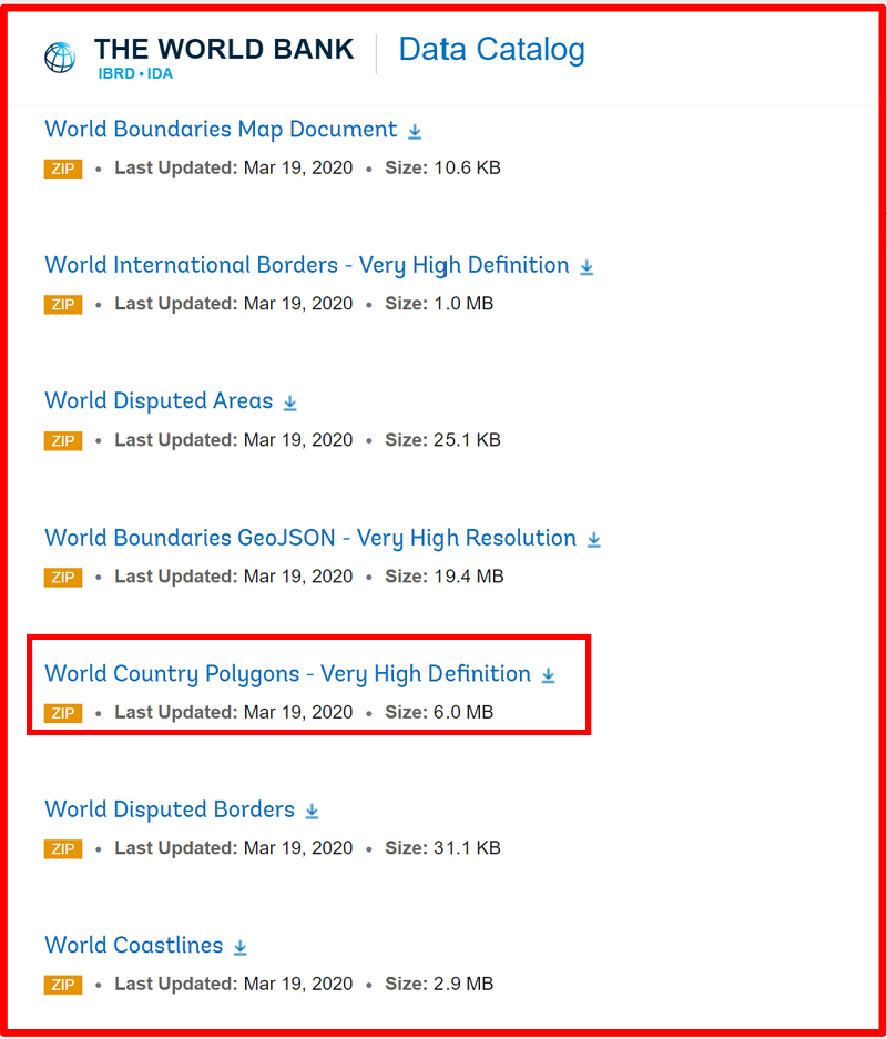
Fig. 4.1.1 Downloading page of the WorldBank

After downloading the file open QGIS and create a new project, to which add the new shapefile (Fig. 4.1.2).

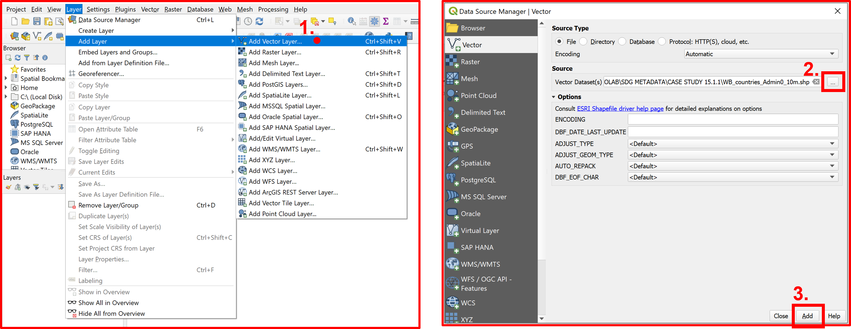
Fig. 4.1.2 Adding a vector layer to QGIS interface

Now we need to extract from the world’s map only the polygon of Suriname. To do so we will use the “Select Features by Area or Single Click” and select Suriname as shown in Fig. 4.1.3.

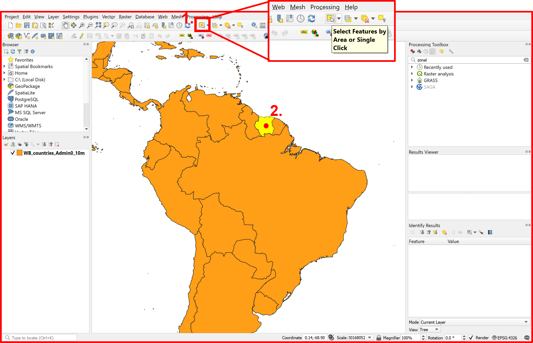
Fig. 4.1.3 Selecting Suriname by area

After selecting Suriname we will want to create a new shapefile containing only this one polygon. To do so we need to Save the selected features in our working directory and name it (Fig. 4.1.4). Make sure that the “Add saved file to map” box is checked.

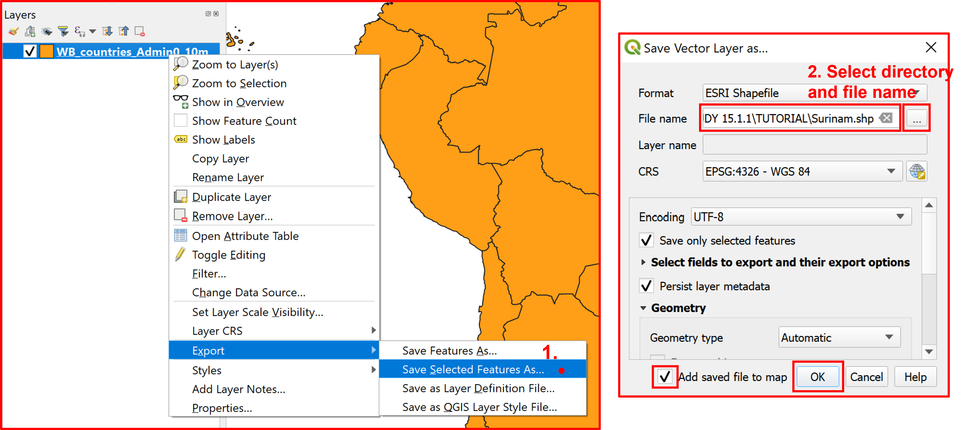
Fig. 4.1.4 Exporting selected features as a new layer

To better visualize the borders of Suriname, change the symbology of the layer. To do so, right click the “Suriname” layer in the layer pane and select “Properties”. After that go to “Symbology” and change it so that the fill color is set to “no brush”, the stroke color is of a bright, contrasting color, and the strike width is quite thick (Fig. 4.1.5).

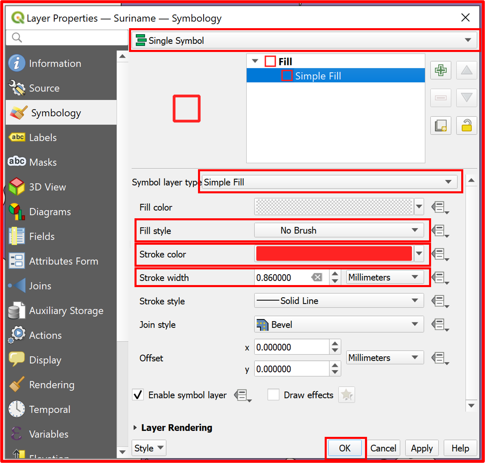
Fig. 4.1.5 Changing the symbology of the new Suriname.shp layer

Now that we have the Suriname polygon, which will serve us to derive the land area for the calculations, it’s time to access the forest data. We will use the Global Land Cover data from https://lcviewer.vito.be/2015. After accessing the website follow the instructions shown in Fig. 4.1.6 to retrieve the forest coverage raster file of the Suriname area.

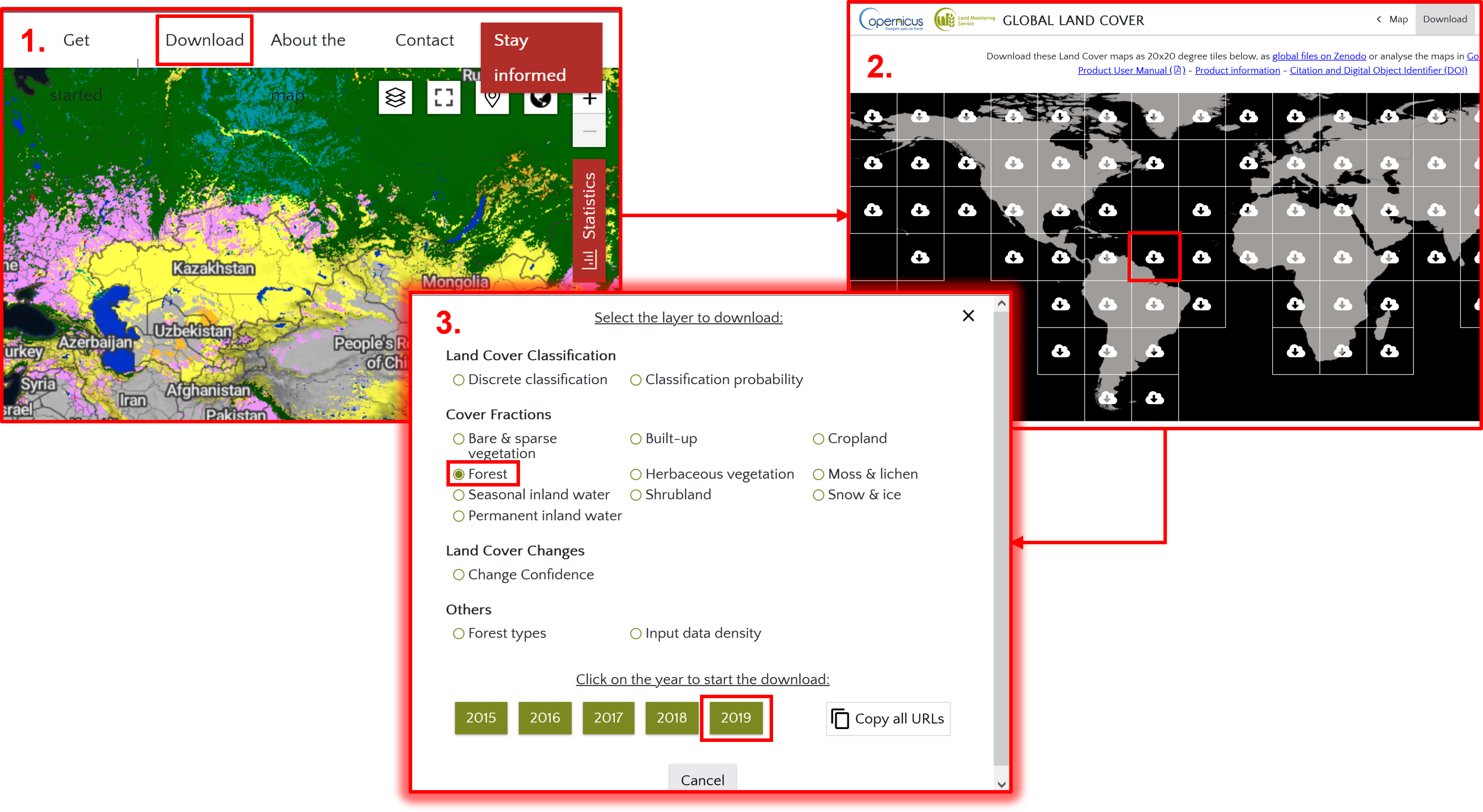
Fig. 4.1.6 Downloading forest data

After downloading the file, add it to the project by using the “Add Raster Layer” function, which you’ll access analogously to the “Add Vector Layer” function presented before.

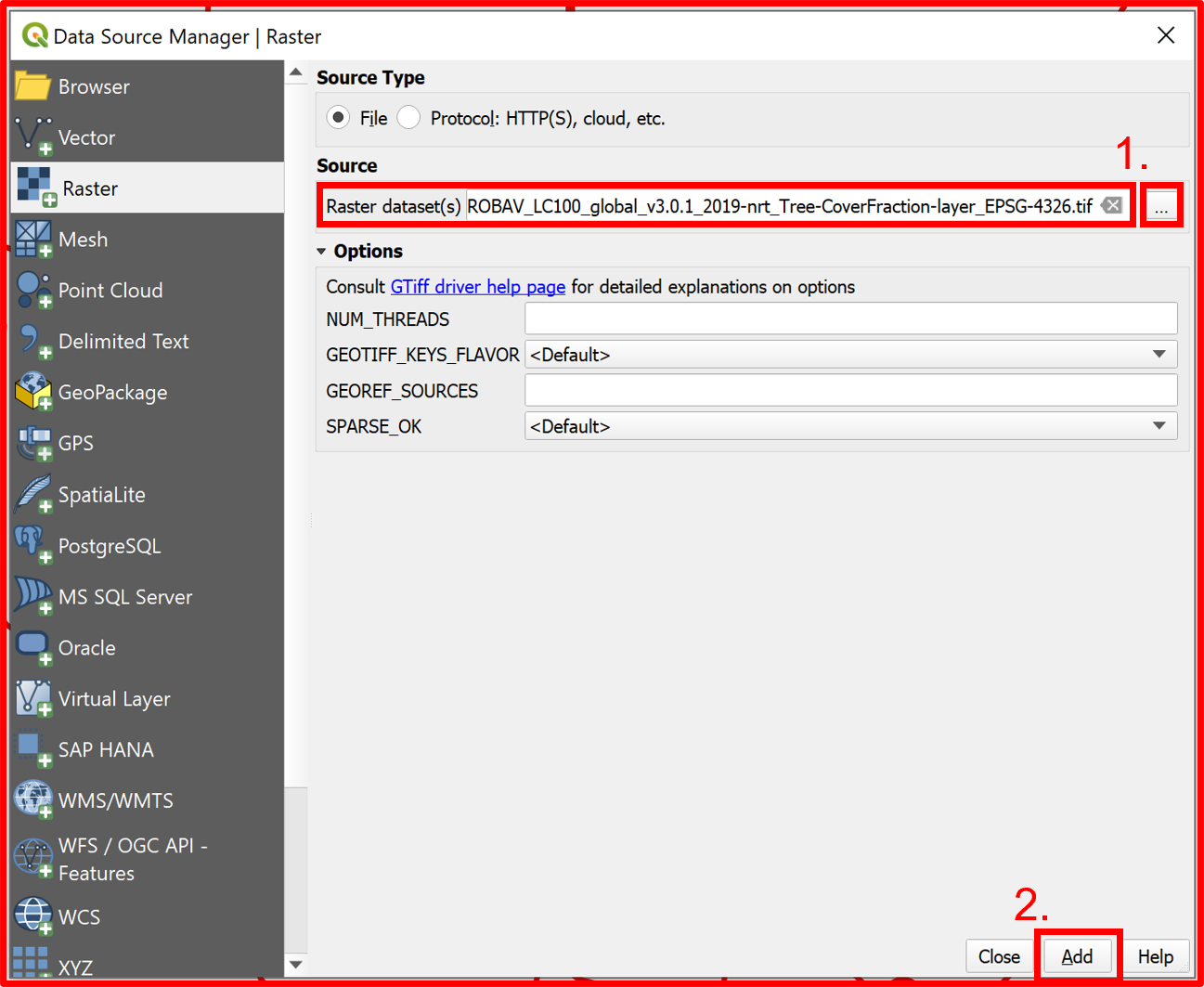
Fig. 4.1.7 Adding the forest raster data layer to the project

After adding the downloaded vector and the raster layer, the view of your project should be similar to the one shown in Fig. 4.1.8.

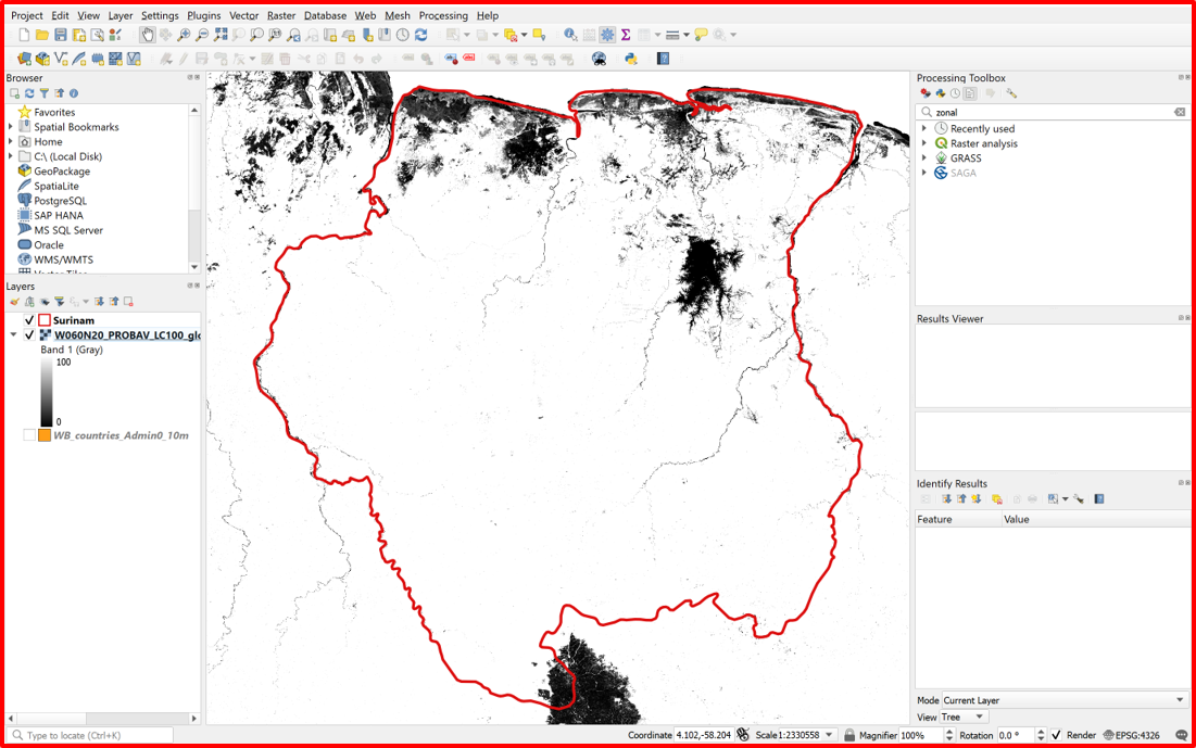
Fig. 4.1.8 Expected layer view after adding both the vector and raster layer

To extract the forest areas of Suriname we need to clip the forest raster layer by mask as shown in Fig. 4.1.9.

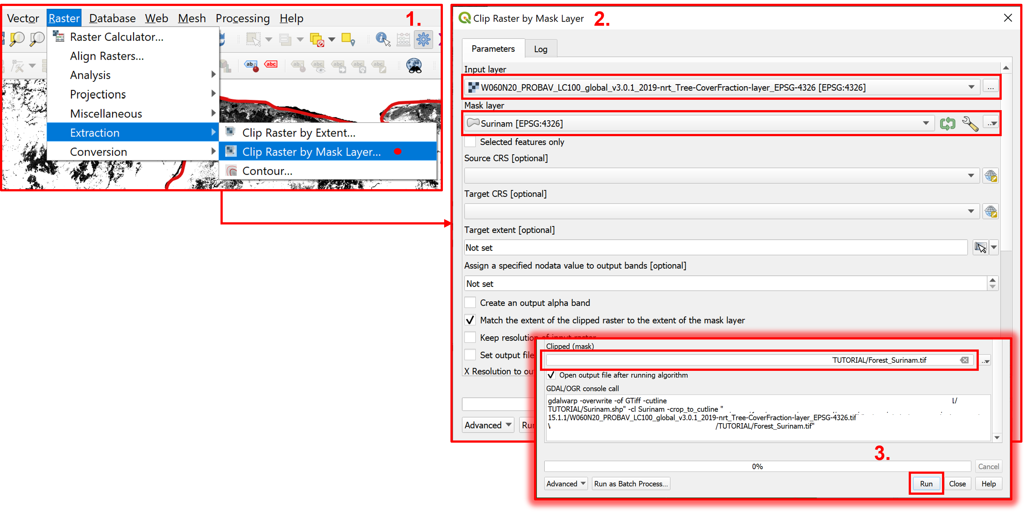
Fig. 4.1.9 Clip forest data raster layer by Suriname vector mask layer

The forest raster layer is a Fractional Cover layer, this means that it gives the percentage of a 100 m pixel that is filled with forest. Pixels have values between 0 and 100, in steps of 1%. Since we just need the information whether the forest is present or not, we will reclassify the layer using the Raster Calculator (Fig. 4.1.10). We’ll classify the pixels with a value equal or bigger than 50% as forest (1) and the rest as no forest pixels (0).

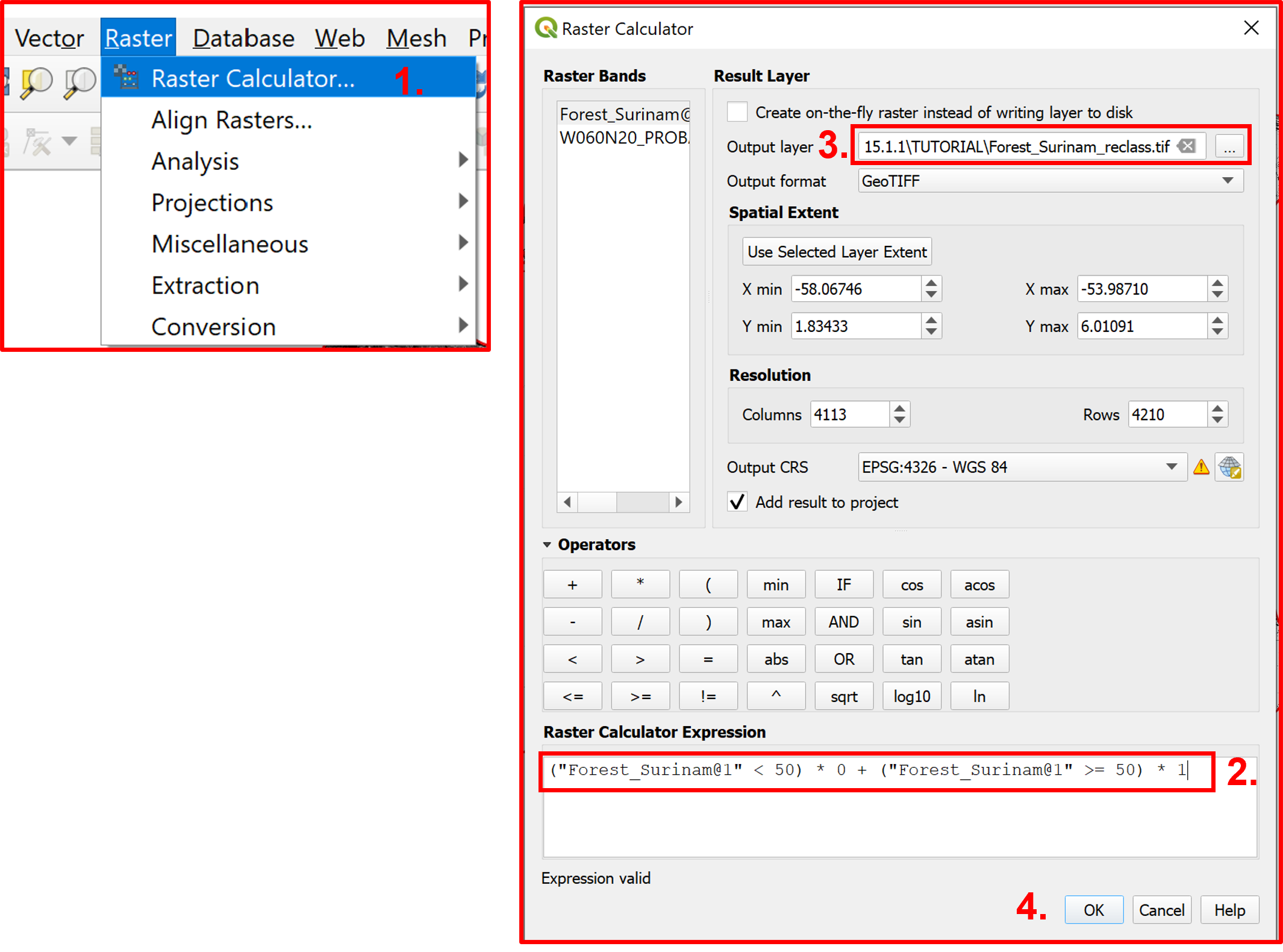
Fig. 4.1.10 Reclassify the clipped raster layer

After reclassifying the raster let’s change the symbology of the new layer for better visualization of the forest area. The expected view after this operation should be as shown in Fig. 4.1.12.

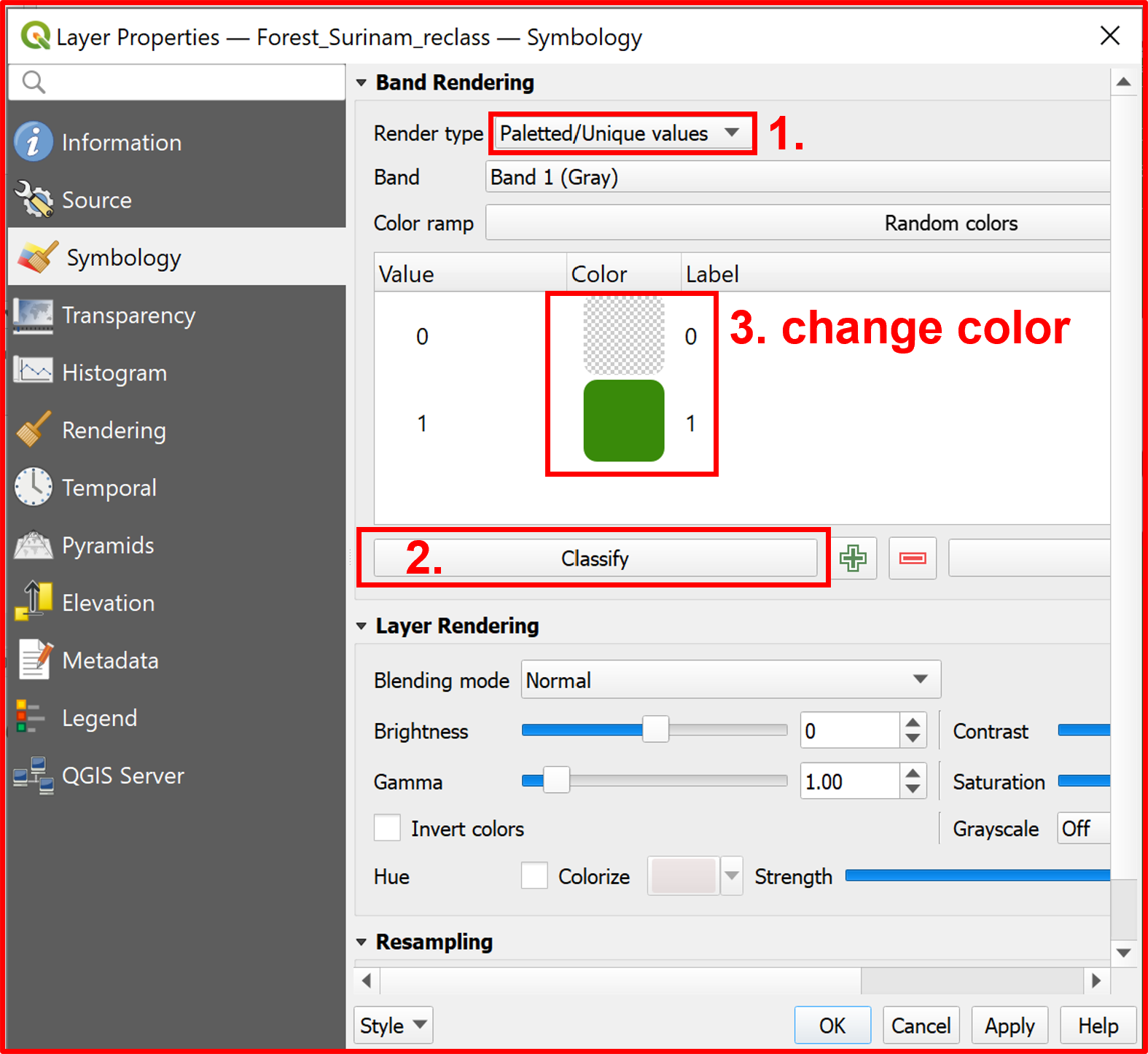
Fig. 4.1.11 Changing the symbology of forest data reclassified raster layer

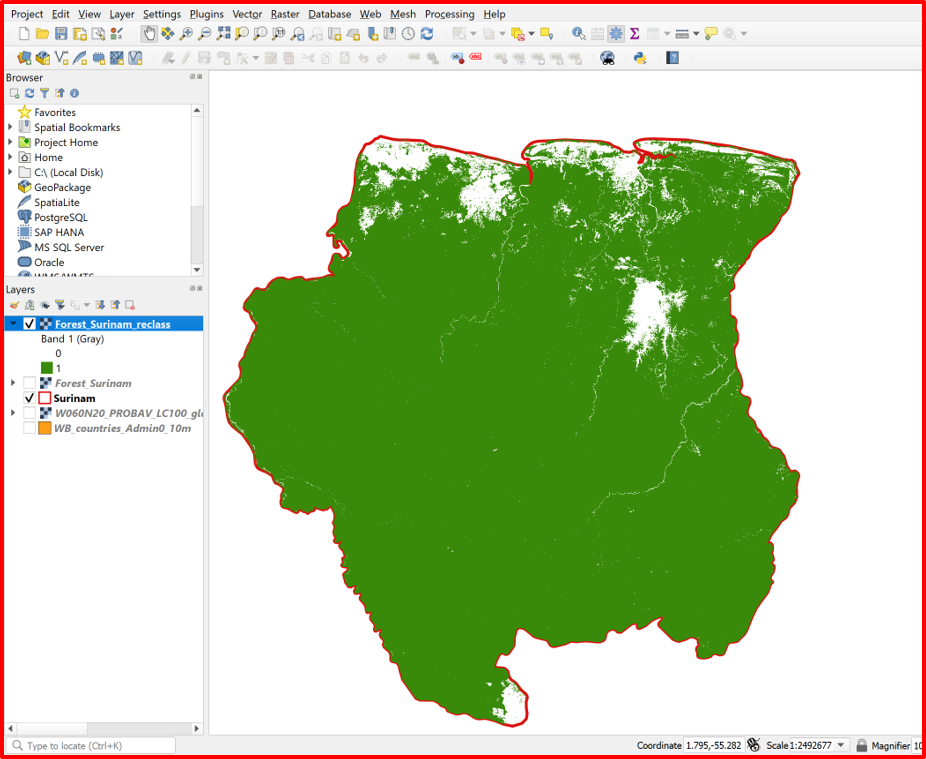
Fig. 4.1.12 Expected layer view after changing the reclassified layer symbology

Since the pixels representing the forest have the value of 1 the sum of all the pixel values will give us the number of forest pixels in the raster file, and knowing the pixel’s size we can calculate the area of the forest in Suriname. To calculate the sum of the pixels values we”ll use the “Zonal Statistics” tool (Fig. 4.1.13).

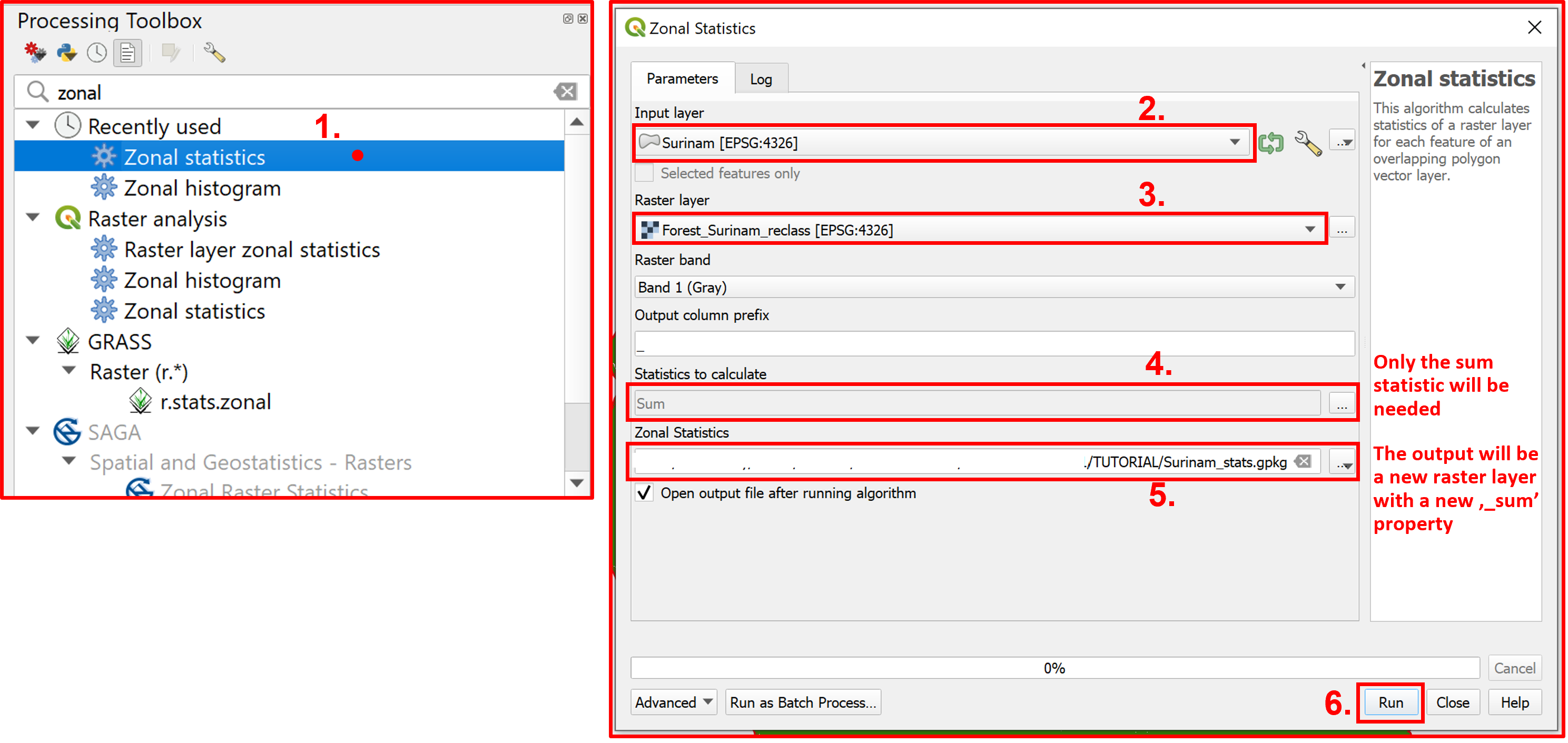
Fig. 4.1.13 Zonal statistics tool

To organize the attribute table we can delete some of the unnecessary columns in the Suriname statistics layer (Fig. 4.1.14). It is not a mandatory step, but it provides a more clear view of the table and makes it easier to work with. The “_sum” column is the result of applying the “Zonal statistics” tool in the previous step.

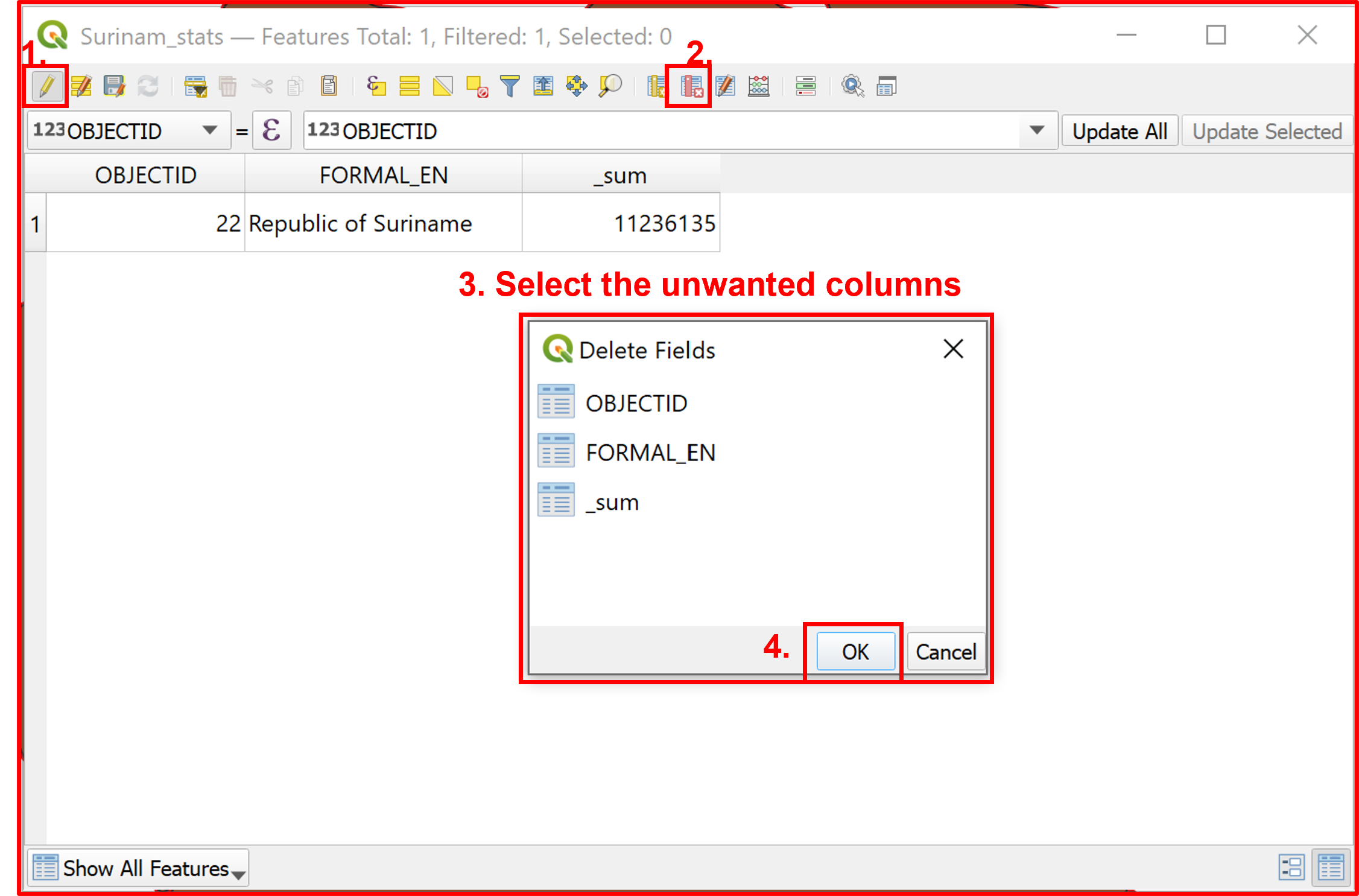
Fig. 4.1.14 Delete the unwanted columns

The last step is to finally calculate the indicator. We have all the required data in the “Suriname_stats” layer. We will use the field calculator to calculate the indicator. Since we now that the pixel size is 100 m x 100 m we will calculate the forest area as: “_sum” * 100 * 100. The land area is given by the built in function “$area”. The exact formula and result is shown in Fig. 4.1.15.

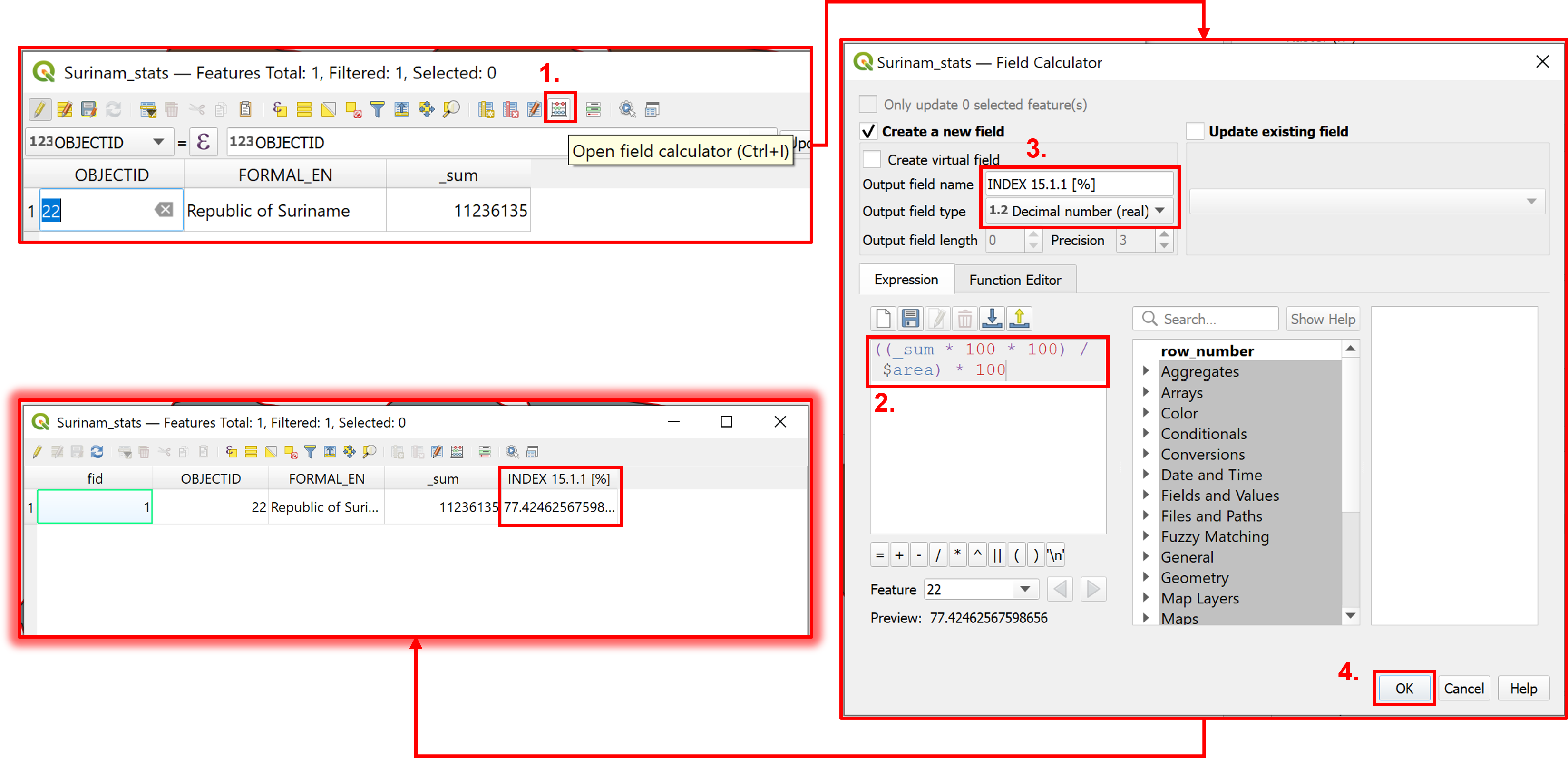
Fig. 4.1.15 Calculate the indicator 15.1.1 using the field calculator

The final result suggests that the forest areas contributed approximately 77.42% of the total land area of Suriname in 2019.